Efficient Benchmarking of NLP APIs using Multi armed Bandits

Efficient Benchmarking of NLP APIs using Multi-armed Bandits

Gholamreza HaffariandTuan TranandMark Carman Faculty of Information Technology, Monash University

Clayton, VICTORIA 3800, Australia

{gholamreza.haffari, mark.carman}@monash.edu [email protected]

Abstract

Comparing NLP systems to select the best one for a task of interest, such as named entity recognition, is critical for practition-ers and researchpractition-ers. A rigorous approach involves setting up a hypothesis testing scenario using the performance of the sys-tems on query documents. However, often the hypothesis testing approach needs to send a large number of document queries to the systems, which can be problematic. In this paper, we present an effective al-ternative based on the multi-armed ban-dit (MAB). We propose a hierarchical gen-erative model to represent the uncertainty in the performance measures of the com-peting systems, to be used by Thompson Sampling to solve the resulting MAB. Ex-perimental results on both synthetic and real data show that our approach requires significantly fewer queries compared to the standard benchmarking technique to identify the best system according to F-measure.

1 Introduction

F-measureAs new NLP systems are (continually) introduced for a task of interest, such as named entity recognition (NER), it is crucial for prac-tioneers and researchers to select the best system. These systems may be designed based on different models and/or learning algorithms. For instance, due to recent advancement in NER research, sev-eral NER systems have been proposed and then supported in APIs such as OpenNLP (Ingersoll et al., 2013), Stanford NER (Finkel et al., 2005), ANNIE (Cunningham et al., 2002) and Meaning Cloud (MeaningCloud-LLC, 1998) to name a few.

Often, the competing NLP systems are bench-marked according to their average performance measure, e.g. F-measure capturing both Precision and Recall, across a set of example documents. Each document produces a single F-measure and the true performance of the system is considered to be the expected value across all possible doc-uments from the domain. Performance on indi-vidual documents correspond to samples from the performance distribution of the system, and can then be used to determine the best system (or set of systems should the highest performing system not be unique) using rigorous hypothesis testing. However, this approach usually requires querying each competing system with a large number of documents, which can be problematic if either the number of test documents is limited, or the sys-tems are implemented as APIs by a third party and performing each query incurs a cost.

In this paper, we present a statistically effective method to identify the best system from a pool of systems. Our approach requires significantly fewer example documents to reach similar guarantees as the traditional hypothesis testing set up, hence re-ducing the cost and increasing the speed of infer-ence. Inspired by the previous work (Scott, 2015; Gabillon et al., 2012; Maron and Moore, 1993), We formulate the benchmarking problem as a se-quential decision process of choosing the best arm as the results of new queried documents are re-ceived. More specifically, our formulation is based on the best arm identification in a multi-armed bandit (MAB) decision process. This allows us to adapt Thompson Sampling (Thompson, 1933) and its variants (Russo, 2016) to efficiently solve the resulting MAB problem.

A crucial difference between the MAB ap-proach and the traditional hypothesis testing is that it is asequentialtesting process, instead of a static testing process which forces the benchmarker to

wait for a final answer at the end of an experi-ment. As such, we need to model the uncertainty regarding the estimated F-measure of each com-peting system, and continually update it as each new document is queried. We propose a novel hi-erarchical model for this purpose, which is gener-ally applicable to document-level evaluation tasks based on F-measure. The inference in our model is done using standard sampling techniques, such as Gibbs sampling.

We analyse empirically the performance of our approach versus the standard hypothesis testing baselines on synthetic datasets as well as real data for the tasks of sentiment classification and named entity recognition. The empirical results confirm that the number of query documents needed to achieve a particular statistical significance level with our approach is much lower than that required by the hypothesis testing baselines.

2 Best Arm Selection in Multi-Armed Bandit

Our aim is to identify the best system among a finite set of systems based on the noisy sequen-tial measurements of their quality. We formulate this problem as the best arm selection in multi-armed bandit. MAB is a sequential decision pro-cess where at each time step n an arm an from the collection of K slot machines is chosen and played by the gambler. Each arma∈ {1, . . . , K} is associated with anunknownreward distribution f(y|θa)from which the reward is generated when the arm is pulled. In the best arm selection prob-lem, the gambler’s goal is to select the arm which has the highest expected reward.

In the common formulation of the MAB, the gambler wants to maximise his cumulative re-wards. Intuitively, maximising cumulative rewards eventually leads to the selection of the best arm since it is the optimal decision. However, (Bubeck et al., 2009) gives a theoretical analysis that any strategies for optimising cumulative reward is sub-optimal in identifying the best performing arm. To this end, several algorithms have been pro-posed for the best arm selection e.g. (Maron and Moore, 1993; Gabillon et al., 2012; Russo, 2016). Although originally developed for maximising cu-mulative rewards, (Chapelle and Li, 2011; Scott, 2015) provide extensive empirical evidence for the practical success of the Thompson Sampling algo-rithm for the best arm selection. In what follows,

we present Thompson Sampling (TS) and one of its variants, called Pure Exploration TS (PETS), designed specifically for the best arm selection.

2.1 Thompson Sampling

Let us denote by (a1, y1), . . . ,(aT, yT) the se-quence of pulled arms and the revealed rewards, atis the arm pulled at time steptandytis its as-sociated reward. Note that this sequence is con-tinually growing as the experiment progresses and new arms are pulled. Let f(y|θa) be the proba-bility distribution to model the unknown reward function of the arma. Had we known the param-eters of the reward functions, the best arm could then be selected as

argmax_aEf(y|θa)[y] = argmaxa

Z

f(y|θa)ydy.

Let us denote the collection of all parameters byΘ := (θ1, . . . ,θK). Assuming a prior over the parameters π0(Θ), we take a Bayesian approach

and reason about the posterior of the parameters:

πT(Θ) = R π0(Θ)LT(Θ)

Θ0π0(Θ0)LT(Θ0)dΘ0

whereΘis the parameter domain, and LT(Θ)is the likelihood of the observed data{(at, yt)}T

1

LT(Θ) := T Y

t=1

f(yt|θat).

The posterior probability that a particular armais optimal (i.e. has the highest expected reward) is:

αT,a:= Z

Θa

πT(Θ)dΘ

whereΘais the set of those parameter values un-der which the armawould be selected as the opti-mal arm:

Θa:={Θ∈Θ|Ef(y|θa) = argmaxa0Ef(y|θ_a0)}

Algorithm 1Pure Exploration TS (PETS)

Initialization: Pull each arm once

t=K

whiletermination condition is not metdo

ˆ

Θ∼πt(Θ)

a←argmax_kE_f(y|θˆk)[y]

r∼uniform(0,1)

ifr≤βthen

Pullaand update the posteriorπt+1(Θ) else

b←a

whileb=ado

ˆ

Θ∼πt(Θ)

b←argmax_kE_f(y|θˆ_k)[y] end while

Pullband update the posteriorπt+1(Θ) end if

t←t+ 1

end while

2.2 Pure Exploration Thompson Sampling

Thompson sampling can perform poorly for the best arm identification problem. The reason is that once it discovers a particular arm is performing well, it becomes overconfident and almost always selects that arm in the future iterations. In case that arm is not the best arm, it takes a long time for the algorithm to divert from it. For example, if αT,a = 90%, then the algorithm selects an arm other than a on average on every 10 iterations, which would make it significantly longer to get to a point whereαT0_,a0 = 95%, i.e. the point where the algorithm terminates with confidence 95% in a different arma0_.

Let αT := (αT,1, . . . , αT,K) be the vector of arm probabilities to be optimal. Pure Explo-ration Thompson Sampling (Russo, 2016) ad-dresses the above deficiency of Thompson Sam-pling by throwing away, with probability β, the arm a sampled from αT. Instead, it samples an-other armb 6=awith the probability proportional toαT,b. The exploration parameterβ prevents the algorithm from exclusively focusing on one arm. Usually β is set to .5 but we empirically inves-tigate other values for this parameter in §4. We can revert to basic Thompson Sampling by setting β = 1in PETS. Similar to Thompson Sampling, this arm selection method can be efficiently im-plemented as shown in Algorithm 1. We terminate the algorithm when it reaches a maximum number of queries or when αT,a ≥ 1−δ, whereδ is the confidence parameter provided in the input.

3 A Probabilistic Generative Model of F-measure

In this section we present a novel hierarchical Bayesian model for capturing the uncertainty over systems’ F-measures, as the prediction outcome on new query documents are received. We present this model for F-measure, however, we note that it can be extended for other performance measures as well.

F-measure is defined as the harmonic mean of the precision and recall:

F-measure := ₁ 2 precision+recall1

precision := _{T P}T P_{+F P} , recall:=_{T P}T P_{+F N}

where (T P, F P, T N, F N) denote true posi-tive, false posiposi-tive, true negaposi-tive, and false neg-ative counts. These counts result from compar-ing the predictions of a system with the ground truth annotations, and they sum to the total number of annotated data items N. We denote the normalised version of the counts by rates ( ˆT P ,F P ,ˆ T N,ˆ F Nˆ ), which are derived by divid-ing the raw counts by N. Importantly, the rate statistics are enough to calculate precision, recall, and F-measure.

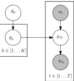
Instead of modelling the uncertainty over the F-measure of a system directly, we model the un-certainty over its rate statistics. Any distribution over( ˆT P ,F P ,ˆ T N,ˆ F Nˆ )then induces a distribu-tion over F-measure. The benefit of working with the rate statistics is that they relate more naturally to the observed(T P, F P, T N, F N)counts, as es-tablished in our generative model in the following. More specifically, we assume a hierarchical model to generate the rate statistics of the sys-tems and the observed (T Pd, F Pd, T Nd, F Nd) counts over a collection of documents d ∈ D. For each system, we draw its rate statisticsθk := ( ˆT Pk,F Pˆ k,T Nˆ k,F Nˆ k) from a Dirichlet prior. To generate the counts statistics resulting from ap-plying the systematon the documentdt, we first generate a document-specific rate vectorµ_dt from a Dirichlet distribution centred aroundθat. Note

that including explicit document-specific ratesµ_dt

in the model (from which the binomial counts are drawn) is necessary in order to allow for sufficient variation in the observed error rates across documents, due to the inherent differences in difficulty of labelling different documents.1

vari-θ0

θk

k∈[1. . . K]

t∈[1. . . T]

cdt

at

µdt

Figure 1: The graphical model for the probabilis-tic generation of a system’s parameters θk and a document’s countscdt, as the selected systemat

is applied onto the documentdtat the time stept. The observed quantities are shaded.

We then generate the observed counts cdt :=

(T Pdt, F Pdt, T Ndt, F Ndt) from the Bionomial

distribution with parameters µ_dt andNdt, where

Ndt is the number data items in dt. In summary,

the generative model is as follows:

∀k∈[1..K] : θk∼Dirichlet(θ0, α0)

∀t∈[1..T] : µ_dt ∼Dirichlet(θat, α)

cdt ∼Bionomial(µdt, Ndt)

whereα0andαare the concentration parameters,

which we set to 1 in our experiments in §4. Fig-ure 1 depicts the graphical model.

For inference, the quantities of interest are the unknown rates for the systems {θk}K_k=1. The observed quantities are document-specific counts {cdt}Tt=1, and we would like to marginalise out the

latent document-specific rate variables{µ_dt}T t=1.

We resort to Gibbs sampling for inference in our model. That is, we iteratively select a hidden vari-able and sample a value from its posterior given all the other variables are fixed to their current values. In our experiments, we collect 1000 samples from the posterior.2_{Algorithm 2 depicts the}

sampling-based inference for the posterior embedded in the PETS algorithm for the best system identification. F-measure is a frequently used evaluation mea-sure, which can straightforwardly be parametrized to allows for varying the importance of precision

ability in (TP,FP,TN,FN) counts, we had to use a Dirichlet-Compound-Multinomial with shared Dirichlet prior rather than a simple Multinomial with a shared Dirichlet Prior.

2_{We make use of the JAGS (Just Another Gibbs Sampler)} toolkit (Plummer, 2003) for inference in our model.

Algorithm 2Identifying the best system

Require: K: Number of arms, J: Number of

sam-ples from posterior π(.), D: Document collection, Fmeasure( ˆT P ,T N,ˆ F P ,ˆ F Nˆ ) := 2 ˆT P

2 ˆT P+ ˆF P+ ˆF N,

NextDoc(a,D): Next document for an armafromD 1: for k∈[1..K]do

2: Dk←NextDoc(k,D)

3: Sk← {˜θj|∀j∈[1..J] : ˜θjGibbs∼ π(θj|Dk)}

4: end for

5: whiletermination condition is not metdo

6: fork∈[1..K]do

7: fk∼ {Fmeasure(˜θ)|θ˜∈ Sk}

8: end for

9: a←argmax_kfk

10: r∼uniform(0,1) 11: b←a

12: ifr > βthen

13: whileb=ado

14: fork∈[1..K]do

15: fk∼ {Fmeasure(˜θ)|˜θ∈ Sk}

16: end for

17: b←argmax_kfk

18: end while

19: end if

20: Db← Db∪NextDoc(b,D)

21: Sb← {θ˜j|∀j∈[1..J] : ˜θjGibbs∼ π(θj|Db)}

22: end while

versus recall:

Fβ-measure:= _β 2

precision+recall1−β

where β is a parameter trading off precision and recall. We note that our approach can be ap-plied straightforwardly to Fβ-measure to put more weight on precision or recall where appropriate.

4 Empirical Results and Analysis

We designed two sets of experiments to exam-ine the efficiency and performance of each algo-rithm using synthetic data as well as real data for sentence level sentiment classification and named entity recognition tasks. With the synthetic data, we analyse our probabilistic generative model for F-measure in combination with the arm selection algorithms. With the real data, we showcase the statistical efficiency of our best system identifica-tion approach compared to the standard hypothesis testing approach (Demˇsar, 2006).

reorderings of the document collection. We em-phasise that, in these experiments, we simulate a scenario where the aim is to select the best system with the minimum number of queries to showcase the effectiveness of our approach.

4.1 Baselines

As baselines, we consider the minimum number of documents needed by the standard statistical power approach. The power of a binary hypothesis testing is the probability that the test correctly re-jects the null hypothesis (H0) when the alternative

hypothesis (H1) is true. In order to find a

lower-bound for the number of documents, we make use of the power calculation for a paired T-Test.

The T-Test indicates whether or not the differ-ence between two groups’ averages most likely re-flects a “real” difference in the population from which the groups were sampled. Assuming we have two competing systems, we can set up a T-Test to assess whether there is a meaningful differ-ence between the F-measures of the two systems.

We assume an efficient experimental design where the same number of (identical) documents are sent to each system. Assuming a typical power setting of 80% and a significance level of 5%, we can calculate an “Oracle baseline” by making use of the true effect size (the standardised difference in mean performance) across the top two systems.3

Obviously this quantity would not be known a-priori of running the experiment, hence the sample size calculated based on this effect size provides a lower-bound on the number of samples that ought be needed4_.

Across the systems, average performance on in-dividual documents will vary due to variations in the inherent difficulty of each document. In other words, some documents are harder to label than others. Thus we make use of a paired sample test for the power calculation. Effect sizes are calcu-lated as follows:

• For the synthetic experiments, the variation in difficulty of the documents is not mod-elled, so we calculate the effect size by sim-ply using the parameters of the simulation as:

3_{For the power calculation, we use the following R} command power.t.test(delta=effect, sd=1, sig.level=0.05, power=.8, type="paired", alternative="one.sided").

4_{Note that the T-Test assumes Gaussian distributed data,} but the violation of this assumption is unlikely to greatly ef-fect the sample size estimates.

µ1−µ2 √

(σ2

1+σ22), whereµ1is the mean performance on the best system andµ2is the mean

perfor-mance on the second best system (likewise for the standard deviationsσ1andσ2.

• For the experiments on real data, variation will be document dependent and hence we calculate the effect size as AV G(f1−f2)

ST DEV(f1−f2), where we directly measure the average and standard deviation of the performance dif-ferences between the top performing APIs across the documents.

Since we are comparing many APIs at once, and a priori of running the experiment we don’t know which two systems are the best, we make use of two settings for the confidence level (aka P-value threshold) for the power calculation:

• Baseline2: Assume the top two systems are

known a priori and use the significance level of 5% directly to produce a lower bound on the number of iterations.

• BaselineK−1:Assume one system is new and

is being compared with all otherk−1APIs. We reduce the required significance level α using a Bonferroni correction to beα/(k−1) to take into account the k−1 comparisons being performed.

We stress that this is an unrealistic scenario in which the effect size is known before running the experiment. If this value is not known or needs to be estimated before the experiment a much larger value would be used, for example a value based on the error thresholdmight be appropriate.

4.2 Synthetic Data Experiments

margin.05 margin.025 margin.01 # queries success% # queries success% # queries success%

Baseline2 120 - 440 - 2725

-BaselineK−1 185 - 680 - 4195

-Hierarchical

+ Thomp. Samp. 22±5 100 41±6 96 66±8 100

+ Pure Eexpl. TS 19±3 100 27±5 100 64±9 96

Gaussian

+ Thomp. Samp. 513±46 100 1169±84 100 2000±0 100

+ Pure Eexpl. TS 360±33 100 848±63 100 1965±19 100

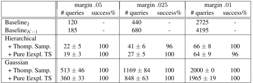
Table 1: Average number of queries across different margins. The number of systems is 5, and the maxi-mum number of queries is set to 2000, andδ= 0.05.

then generated based on our generative model. For each competing configuration, we repeat the experiment multiple times in order to account for the randomness inherent in the algorithms and the generated documents. In different experiments, we let the number of competing systems K be {5,10,20}.

Margin and the number of systems. In this experiment, we investigate the relation between the margin and the number of documents queried by each algorithm. Intuitively, as the margin between the top performing systems decreases, more queries are required to segregate the best system among the top performing ones. We run each algorithm for 500 times on the competing configurations for each margin withK = 5. The maximum number of queries allowed is 2000, and the algorithm can terminate earlier as soon as αT,a≥.95, i.e.δ= 0.05.

Table 1 summarises the average number of queries and the success rates of TS and PETS in combination with our hierarchical Bayesian model for F-measure across different margins. We see that the number of query documents increases as the margin decreases. It is also worth noting that PETS requires slightly smaller number of queries than Thompson Sampling. Interestingly, the num-ber of samples required by the hypothesis testing baselines is much more than that required by the TS/PETS combined with our hierarchical model.

We then ask the question whether the number of competing systems is important. Table 2 summarises the average number of queries and the success rate of each algorithm on the competing configurations for the margin 0.05 for varying number of systemsK ∈ {5,10,20}. As seen, the

number of queries increases (sub)linearly with the number of competing systems.

Hierarchical vs Gaussian.We compare our hier-archical model for capturing the uncertainty over F-measure with the Gaussian distribution. That is, we associate a Gaussian distribution to each sys-tem to model its posterior over the F-measure. The use of the Gaussian distribution to model the mean of sampled F-measures is motivated by the law of large numbers. This approach directly models the uncertainty of a system’s F-measure, as opposed to our indirect modelling approach where posterior distribution is constructed using the distribution of ( ˆF P ,F N,ˆ T P ,ˆ T Nˆ )rates.

Tables 1 and 2 show the average number of queries and success rates for algorithms using our hierarchical model vs the Gaussian distribu-tion based model. The general trend is that using the Gaussian model in TS/PETS requires signif-icantly more queries compared to the hierarchi-cal model as well as the baselines. Needing more queries compared to the baselines highlights the importance of choosing the right distribution for capturing the uncertainty over the F-measure in TS/PETS. Needing more queries compared to the hierarchical variant is somewhat expected as the synthetic data is generated according to the hierar-chical model. However, we will see similar trends in the experiments on the real data.

4.3 Sentiment Analysis

K: 5 K: 10 K: 20

# queries success% # queries success% # queries success%

Baseline2 120 - 245 - 400

-BaselineK−1 185 - 380 - 620

-Hierarchical

+ Thomp. Samp. 22±5 100 43±6 96 70±14 100

+ Pure Eexpl. TS 19±3 100 35±5 100 64±13 100

Gaussian

+ Thomp. Samp. 513±46 100 1019±59 100 1404±75 100

+ Pure Eexpl. TS 360±33 100 661±38 100 937±62 100

Table 2: Average number of queries across different number of competing systems. The margin is 0.05, and the maximum number of queries is set to 2000, andδ = 0.05.

to a patient.

Dataset. We make use of a biomedical cor-pus (Martinez et al., 2015) consisting of CT reports for fungal disease detection collected from three hospitals. For each report, only the free text section were used, which contains the radiolo-gist’s understanding of the scan and the reason for the requested scan as written by clinicians. Every report was de-identified: any potentially identifying information such as name, address, age/birthday, gender were removed. There are a total of 358 test documents, where the average number of sentences per document is 23.

Competing Systems.We make use of a variant of the coarse-to-fine model proposed in (McDonald et al., 2007) for sentiment analysis. Briefly speaking, the model couples the sentiment of the sentences contained in a report with the overall sentiment of the report. We train four versions of the model, each of which corresponds to a different training condition:

• Mfull: where the model is trained on the fully

annotated dataDF, i.e. the data annotated at both the sentence and report level.

• Mpartial: where the model is trained on both

DF and the partially annotated data DP in which the sentence level annotation is miss-ing but the reports are labeled.

• Munlab: where the model is trained onDF and

DUin which the annotation is missing at both sentence and report level.

• Mall: where the model is trained on all of the

available data described above.

# queries % success

Baseline2 856

-BaselineK−1 1320

-Hierarchical

+ Thomp. Samp. 152±36 100 + Pure Eexpl. TS 123±37 100 Gaussian

+ Thomp. Samp. 500±0 100 + Pure Eexpl. TS 500±0 100

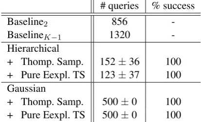
Table 3: Sentiment classification for biomedical reports with 4 competing models. The maximum number of queries is set to 500, andδ= 0.05.

We expect Mall to outperform the other models.

The aim is to analyse the behaviour of our best system selection methods on real data compared to the baselines.

Results. Table 3 presents the results. As seen the number of queries needed for the TS/PETS combined with the hierarchical model is much less than that of the baselines and the Gaussian variant.

4.4 Named Entity Recognition

In our second set of experiment, we attempt to see how our frameworks and F1 models perform

using realistic data.

Open American National Corpus (OANC). This corpus includes a wide variety of linguistic anno-tations with a balanced selection of texts from a broad range of genres/domains. The diversity of the corpus will enable us to assess the robustness of tools across different domains. The number of documents in the MASC corpus is about 392.

Competing Systems. We evaluate the per-formance of 5 popular NER systems implemented as API in third party implementations:

• OpenNLP (Ingersoll et al., 2013): The Apache OpenNLP library is a machine learn-ing based toolkit for the text processlearn-ing. It is based on the maximum entropy and percep-tron.

• Stanford NER (Finkel et al., 2005): It is based on linear chain Conditional Random Field (CRF) sequence models. It is part of the Stan-ford CoreNLP, which is an integrated suite of NLP tools in Java.

• ANNIE (Cunningham et al., 2002): ANNIE uses gazetteer-based lookups and finite state machines for entity identification and classifi-cation. It can recognise persons, locations, or-ganisations, dates, addresses and other named entity types. ANNIE is part of the GATE framework. It can be used as a Web Service but it also provides its own interface for inde-pendent use.

• Meaning Cloud (MeaningCloud-LLC, 1998): It is based on a hybrid approach combining machine learning with a rule based system. The software is available as a cloud based so-lution and on-premise as a plugin module for the GATE framework.

• LingPipe (Alias-i, 2008): It is a set of Java libraries developed by Alias-I for NLP. The NER component is based on a 1st-order Hid-den Markov Model with variable-length n -grams as the feature set and uses the IOB an-notation scheme for the output.

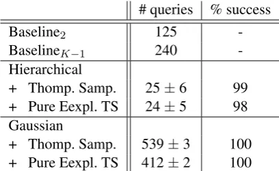
Results.Table 4 presents the results. As seen the number of queries needed for the TS/PETS com-bined with the hierarchical model is much less than that of the baselines and the Gaussian vari-ant.

# queries % success

Baseline2 125

-BaselineK−1 240

-Hierarchical

+ Thomp. Samp. 25±6 99

+ Pure Eexpl. TS 24±5 98 Gaussian

+ Thomp. Samp. 539±3 100 + Pure Eexpl. TS 412±2 100

Table 4: Named entity recognition on MASC doc-uments with 5 competing systems. The maximum number of queries is set to 2000, andδ=.05.

5 Conclusion

We have presented a novel approach for bench-marking NLP systems based on the multi-armed bandit (MAB) problem. We have proposed a hier-archical generative model to represent the uncer-tainty in the performance measures of the compet-ing systems, to be used by the Thompson Sam-pling algorithm to solve the resulting MAB prob-lem. Experimental results on both synthetic and real data show that our approach requires sig-nificantly fewer queries compared to the stan-dard benchmarking technique to identify the best system according to F-measure. Future work in-cludes applying our approach to other NLP lems, particularly emerging document-level prob-lem settings such document-wise machine transla-tion.

Acknowledgments

G. H. appreciates fruitful discussions with Mohammad Ghavamzadeh and Yasin Abbasi-Yadkori. We are grateful to reviewers for their in-sightful feedback and comments.

References

Alias-i. 2008. Lingpipe. Available at: http://alias-i.com/lingpipe.

S´ebastien Bubeck, R´emi Munos, and Gilles Stoltz. 2009. Pure exploration in multi-armed bandits prob-lems. In International conference on Algorithmic learning theory, pages 23–37. Springer.

Hamish Cunningham, Diana Maynard, Kalina Bontcheva, and Valentin Tablan. 2002. GATE: A Framework and Graphical Development Envi-ronment for Robust NLP Tools and Applications. In Proceedings of the 40th Anniversary Meeting of the Association for Computational Linguistics (ACL’02).

Janez Demˇsar. 2006. Statistical comparisons of clas-sifiers over multiple data sets. J. Mach. Learn. Res., 7:1–30, December.

Jenny Rose Finkel, Trond Grenager, and Christopher Manning. 2005. Incorporating non-local informa-tion into informainforma-tion extracinforma-tion systems by gibbs sampling. InProceedings of the 43rd Annual Meet-ing on Association for Computational LMeet-inguistics, pages 363–370. Association for Computational Lin-guistics.

Victor Gabillon, Mohammad Ghavamzadeh, and Alessandro Lazaric. 2012. Best arm identification: A unified approach to fixed budget and fixed confi-dence. InAdvances in Neural Information Process-ing Systems, pages 3212–3220.

Nancy Ide, Collin Baker, Christiane Fellbaum, and Charles Fillmore. 2008. Masc: The manually an-notated sub-corpus of american english. InIn Pro-ceedings of the Sixth International Conference on Language Resources and Evaluation (LREC. Cite-seer.

Grant S Ingersoll, Thomas S Morton, and Andrew L Farris. 2013. Taming text: how to find, organize, and manipulate it. Manning Publications Co.

Oded Maron and Andrew W Moore. 1993. Hoeffd-ing races: AcceleratHoeffd-ing model selection search for classification and function approximation. Robotics Institute, page 263.

Ryan McDonald, Kerry Hannan, Tyler Neylon, Mike Wells, and Jeff Reynar. 2007. Structured mod-els for fine-to-coarse sentiment analysis. In Pro-ceedings of the 45th Annual Meeting of the Associ-ation of ComputAssoci-ational Linguistics, pages 432–439, Prague, Czech Republic, June. Association for Com-putational Linguistics.

MeaningCloud-LLC. 1998. Meaning Cloud. Avail-able at: https://www.meaningcloud.com/.

Martyn Plummer. 2003. JAGS: A program for analysis of Bayesian graphical models using Gibbs sampling. InProceedings of the 3rd International Workshop on Distributed Statistical Computing.

Daniel Russo. 2016. Simple bayesian algo-rithms for best arm identification. arXiv preprint arXiv:1602.08448.

Steven L Scott. 2015. Multi-armed bandit experiments in the online service economy. Applied Stochastic Models in Business and Industry, 31(1):37–45.