Abstract—We have used the semi-parametric Cox proportional hazard regression model to estimate the microarray genes' survival significance and disease classification. We have developed a novel method that estimates the optimal partition (cut-off) of a single gene’s expression level by maximizing the separation of the survival curves related to the high- and low- risk of the disease behavior. Then, we extend our approach to construct two-gene signatures, which can exhibit synergetic influence on patient survival. We demonstrate the utility of our method on two Affymetrix U133 breast cancer patient cohorts. We reveal a large number of genes/gene-pairs providing pronounced synergistic effect on patient’s survival time and identifying patients with low-risk and high-risk disease sub-types. We demonstrate that, among others, MELK-UQCRC1 and AP2S1-KARS gene pairs have a strong clinically-significant interaction effect in survival of the breast cancer patients. Our technique has the potential to be a powerful tool for classification, prediction and prognosis of cancers and other complex diseases.
Index Terms— Cox proportional hazards model, data-driven grouping, synergetic pairs, breast cancer patients’ grouping.
I. INTRODUCTION
Global gene expression profiles of cell transcriptomes, measured by DNA microarrays, are used to diagnose and classify human cancers into genetic sub-types related to different clinical outcomes, as well as to assign appropriate treatment to cancer patients [1]-[3]. These decision-making processes often involve class comparison analysis, which leads to the better understanding of the disease process by identifying gene expression changes in primary tumors associated with patient survival outcomes [1],[2],[4],[5]. An equally important task is class prediction, which improves disease prognosis and treatment prediction by the construction of the so-called “significant gene signature(s)”, that is, gene set(s) that provide a distinction of the given classes of patients at the given level of erroneous predictions [5],[6]. Though different, these two processes share a common gene selection step, which may be more crucial than the significant gene signature modeling or the multiple comparison procedure considered [2],[5]. At the primary stages of identification of the high- and low- risk patients, the selection of “optimal” individual and “synergetic” genes (gene pairs) that significantly correlate with patient’s survival may provide new and very important information on pathogenesis and etiology and further aid in the search for new molecular targets for drug design and therapy.
We discuss a novel computational method to identify the groups of patients with different disease recurrence risk. The method is an extension of our data-driven grouping method described in [7]. The primary goal of data-driven grouping is
to estimate the optimal partition (cutoff) of a single gene’s expression level by maximizing the separation of the survival curves related to high-risk and low-risk of the disease behavior. We further extend this approach to construct two-gene signatures, which can exhibit synergetic influence on patient survival. Using bootstrapping and statistical modeling, we evaluate the performance of our method by analyzing two Affymetrix U133 breast cancer patient cohorts, each consisting of 44,928 transcripts (approximately 30,000 genes). We reveal a large number of gene pairs, which provides pronounced synergetic effect on patient’s survival time and identify patients with low-risk and high-risk disease sub-types. The selected survival significant genes are strongly supported by Gene Ontology (GO) analysis and literature data. We develop an approach to combine the patients’ grouping results from different synergetic genes and gene-pairs into one composite patients’ grouping scheme that further improves the separation of low-risk versus high-risk patients. Our composite grouping correlated strongly with available clinical data (cancer subtype and clinical grades). Finally, we propose an extension to identify three distinct patient groups.
The idea of gene pairs has been successfully used previously for diagnostics and prognosis. In contrast to our work, several studies only used survival modeling for validation of selected gene pairs ([8] and [9]). Ref. [8] carried out the Predictive Interaction Analysis to examine whether any of the gene pairs generated from pre-selected genes (only 300 single genes) of follicular lymphoma were able to discriminate the 5-year outcomes more reliably than either single gene of the pair. Only gene pairs with P values 10 times smaller than the P value of their respective gene members were considered for further analysis. It was found that a high HOXB13/IL-17BR expression ratio is associated with increased relapse and death in node-negative, ER-positive breast cancer patients treated with tamoxifen [9]. However, the 303 gene pairs that passed that criterion were formed by only 15 unique genes due to redundant features or genes represented by multiple probes on the array. This case study suggested that appropriate gene pairs may identify patients in whom alternative therapies should be studied.
II. DATA AND METHODS
A. Survival analysis with Cox proportional hazards model
One of the most popular survival models is the Cox proportional hazards model [10]:
log (1)
Genome-Scale Identification of Survival
Significant Genes and Gene Pairs
where t is survival time, h(t) represents the hazard function, α(t) is the baseline hazard, β is the slope parameter of the model to be estimated and x is the regressor. In our work the regressor is a dummy variable denoting the patients’ groups. Fitting this model we attempt to estimate whether the groups have statistically different survival hazards. This can be evaluated by testing the significance of the β coefficient.
The popularity of this model is due to the fact that it leaves the baseline hazard function α(t) unspecified (no distribution is assumed) and can be estimated iteratively by the method of partial likelihood of [10]. The Cox proportional hazards model is semi-parametric because while the baseline hazard can take any form, the covariates enter the model linearly. It is showed that β coefficient can be estimated efficiently by minimizing the Cox partial likelihood function:
∏ ∑
(2) where R(t) = {j: tj ≥ t} is the risk set at time t and e is the clinical event at time t. The likelihood (2) is minimized by the Newton-Raphson optimization method for finding successively better approximations to the roots of a real-valued function [11]. The estimation is carried out in R using survival package.
B. Selection of Prognostic significance genes
Assume a microarray experiment with i = 1, 2, ..., N genes, whose intensities are measured for k = 1, 2, ..., K breast cancer patients. The log-transformed intensities of gene i and patient k are denoted as yi,k. Associated with each patient k are a disease free survival time tk (DFS time) and a nominal clinical event ek (DFS event) taking values 0 in the absence of tumor metastasis at tk or 1 in the presence of tumor metastasis at time tk. Additional information utilized in this work includes patients histologic grade (1, 2a, 2b and 3) and cancer subtype (Basal, ERBB2, Luminal A, Luminal B, No subtype, Normal-Like), extensively discussed in [2].
Without loss of generality, we define that given gene i
patient k is assigned to the high-risk or the low-risk group by:
1 "# $ %"&', ") *,+ ,
0 ./0 $ %"&', ") *,1 ,
2
(3)
where ci denotes the predefined cutoff of the ith gene’s expression level. After specifying , the DFS times and events are subsequently fitted to the patients’ groups by the Cox proportional hazard regression model:
log 34, 5 (4) where, as before, βi is the parameter to be estimated for each
gene i. To assess the ability of each gene to discriminate the patients into two distinct genetic classes, the Wald statistic (W) [10] of the βi coefficient of model (4) is estimated by
using the univariate Cox partial likelihood function (2). The Wald statistic for βi can be derived as 6 78⁄9:%7. Alternatively, we can estimate the Wald P value for βi as:
< $ 9:.=> Pr ADEFBC B+ GH
8I (5)
where GH8 denotes the chi-square distribution with ν degrees of freedom. Typically, ν is the number of parameters of the Cox proportional hazards model and in our case ν = 1. Expression (5) can be derived from the proper statistical tables of the chi-square distribution. The genes with the lowest βi Wald P values are assumed to have better group
discrimination ability and thus called survival significant genes. These genes are selected for further confirmatory analysis or for inclusion in a prospective gene signature set.
From (3) notice that the selection of prognostic significant genes relies on the predefined cutoff value ci that separates the low-risk from the high-risk patients. The simplest cutoff basis is the mean of the individual gene expression values within samples [6], although other choices (e.g. median, trimmed mean, etc) could be also applied. Two problems, associated with such cutoffs and discussed in details in [7], are: 1) they are suboptimal cutoff values that often provide low classification accuracy or even miss existing groups; 2) the search for prognostic significance is carried out for each gene independently, thus ignoring the significance and the impact of genes' co-expression on the patient’ survival.
To solve problem 1), we develop a data-driven “goodness-of-split” method (DDg) that identifies the optimal partition of patients by model (4). In [7] we compared the performances of mean-based and our data-driven partition and showed the superiority of the latter approach. We also propose a solution to problem 2) by attempting to identify sets of survival significant gene pairs, which can further improve the accuracy of the patients’ classification.
C. Patients and tumor specimens
The clinical characteristics of the patients and the tumor samples of Uppsala and Stockholm cohorts are summarized in [2]. Stockholm cohort comprised of Ks = 159 patients with breast cancer, operated in Karolinska Hospital from 1 January 1 1994 to 31 December 1996, identified in the Stockholm-Gotland breast Cancer registry. Uppsala cohort involved Ku = 251 patients representing approximately 60% of all breast cancers resections in Uppsala County, Sweden, from 1 January 1987 to 31 December 1989. Information on patients' disease-free survival (DFS) times/events and the expression patterns of approximately 30,000 gene transcripts (representing N = 44,928 probe sets on Affymetrix U133A and U133b arrays) in primary breast tumors were obtained from National Center for Biotechnology Information (NCBI) Gene Expression Omnibus (GEO) (Stockholm data set label is GSE4922; Uppsala data set label is GSE1456). The microarray intensities were calibrated by the Robust MultiChip Average (RMA) of [12] and the probe set signal intensities were log-transformed and scaled by adjusting the mean signal to a target value of log500 [2].
D. One dimensional (1D) data-driven grouping
For each gene i, we compute the 10th quantile ( i q10 ) and the 90th quantile ( i
q90) of the distribution of the Ksignal intensity values. Within ( i
q10, i
q90), we search for the cutoff value ci that most successfully discriminates the two unknown genetic classes, which corresponds to the minimum
1. Form the sequence 0KLM 0K &, z = 1, ..., (Q-1), where
0M NMO , 0P NQO and s is a sufficiently small number (e.g. s = 0.02) so that typically 400 ≤ Q ≤600. For i = 1 and z = 1, …, (Q-1) use iteratively
1 "# $ %"&', ") *,+ ,
0 ./0 $ %"&', ") *,1 ,
2
to separate the K patients with , 0K.
2. Using this cutoff, evaluate the prognostic significance of gene i by estimating the K from
log 34, 5 K
The “optimal” cut-off for each i is the one with the minimum JKP value, provided that the sample size of each group is sufficiently large (formally above 25) and model Cox proportional hazards model is plausible. 3. Iterate steps 1-2 for i = 2, ..., N.
E. Two dimensional (2D) data-driven grouping
We generalize the above procedure to consider synergism between genes. Our approach resembles the idea of Statistically Weighted Syndromes algorithm of [6], which classifies the objects (patients) of a training set using “informative” pairs of covariates (gene pairs). We will show that it provides the most accurate discrimination of the patients in terms of the Wald P values of βι. For a given gene
pair i = 1, j = 2 with individual cutoffs ci and cj, i≠j, we may classify the K patients by the seven possible two-group designs of Fig. 1.
Fig 1. Grouping of a synergetic gene pair (genes 1 and 2 with respective cutoffs c1
and c2
) and all possible two-group designs (Designs 1-7).
The letters “A”, “B”, “C” and ”D” are defined by the conditions: A: yi,k < ci and yj,k < cj; B: yi,k ≥ ci and yj,k < cj; C:
yi,k < ci and yj,k ≥ cj; D: yi,k ≥ ci and yj,k ≥ cj. On the basis of this notion, our synergy algorithm works as follows:
1. For i = 1 and j = 2, group the K patients by each of the seven designs of Fig. 1 (using individual gene cutoffs), fit model (4) for each design and estimate the seven Wald P values for βi. Provided that the respective groups sample
sizes are sufficiently large and the assumptions of model (4) are satisfied, the best grouping scheme among the five “synergetic” (1 – 5) and the two “independent” (6 – 7) designs is the one with the smallest βi P value.
2. Iterate 1 for all i and j combinations of the N genes (i = 1, …, N - 1, j = i + 1, …, N).
F. Residuals bootstrap of Cox proportional hazards
To validate the significance of our findings (in terms of the estimated Wald P values) we bootstrap our samples (from the
two cohorts) and estimate 99% confidence intervals for the βi
coefficients of the Cox proportional hazards model. We use the non-parametric residuals bootstrap of [13] using the boot
package in R. Specifically, the algorithm works as follows: 1. Estimate βi of model (4) by maximizing the likelihood (2).
2. Calculate the independent and identically (Uniform in [0,1]) distributed generalized residuals, calculated in [14] by the “probability scale data”:
= R1 $ SOT UVB, k = 1, 2, …, K
where SO WX 1 | exp] 1 denotes the baseline failure time distribution. Typically, S^O is a step function with jumps at the observed failure times (estimated by the survival package), which does not affect the Uniformity of the generalized residuals [14].
3. Consider the pairs _=M, >M, … , =a, >aband resample with replacement B pairs of observations (B bootstrap samples) c3=Md, >Md5, … , 3=ad, >ad5e, b = 1, …, B 4. Calculate the probability scale survival times
d 1 $ R=dTM ⁄ BVB
and estimate the bootstrap coefficients M, 8,..., f by numerically maximizing the partial likelihood (2) for each b = 1, …, B.
5. Based on these coefficients, estimate the Bias-Corrected accelerated (BCa) bootstrap confidence intervals for each βi coefficient that correct the simple quantile intervals of
βi for bias and skewness in their distribution [15].
III. RESULTS
A. One dimensional (1D) data-driven grouping
We correlate gene expression profiles with clinical outcome (DFS time) in the two cohorts and identify specific genes that predict survival among the patients. Our results show that a large fraction of genes could be used to predict survival. On the basis of the training data of each cohort (Fig. 1), we estimate the data-driven cutoffs for each gene.
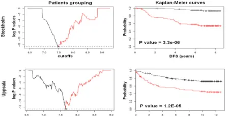
Fig. 2. Plot of log P values against cutoff levels (left) and Kaplan-Meier curves (right) for the MELK prognostic gene in the Stockholm (top) and Uppsala (bottom) cohorts. Black lines indicate the low-risk group and red lines the high-risk group.
[image:3.612.71.300.423.502.2] [image:3.612.316.540.538.653.2]Comparison with the mean-based method is given in [7]. Data-driven grouping provides significant improvements on the prediction of patients’ survival.
Generalizing for the set of 44,928 transcripts, data-driven grouping found 11,107 prognostic significant probesets by Wald test. Next we applied our residuals bootstrap method to further validate our findings thus reducing our survival significant list to 8665 probesets (approximately 78% of the Wald survival significant genes were validated by bootstrap).
In such a large scale experiment, we naturally expect several false positive genes, which we would like to exclude from further analysis. A popular approach to reduce Type I error is to estimate the False Discovery Rate (FDR), initially developed by [16] for independent and positively correlated test statistics (positive regression dependence assumption). An easy way to check these assumptions is to estimate the variance-covariance matrix among all transcripts of the study. If the covariance elements are all positive then the positive regression dependence hold and the original FDR can correct for multiple testing. If not, the general regression dependence holds and [17] suggest using a corrected FDR P value estimated as ∑ M
g log h i j
[image:4.612.65.300.485.567.2]kM , where m denotes the number of tests and γ ≈ 0.57721 is the Euler-Mascheroni constant. The FDR adjustment of [17] is conducted in the R package brainwaver. It produces an FDR threshold against which the Wald P values are tested for significance (if P value ≤ FDR threshold the gene is survival significant). By correcting for multiple testing at corrected P value = 2.0E-04, we resulted in 1,677 survival significant genes in Stockholm. We applied the same series of methods in Uppsala and identified 9,426 Wald survival significant probesets, which were reduced to 1,039 after BCa confidence intervals and FDR correction (P value = 2.2E-04). We claim that the selected probesets of each cohort are highly survival significant and powerful in discriminating patients’ into two survival groups.
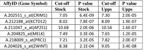
Table I. Top-level survival significant genes
B. Functional significance and reproducibility
We check the functional significance and functional reproducibility of the results in the two cohorts. We seek for common survival significant probesets across the two independent cohorts in terms of Wald statistics, 1% BCa confidence intervals and FDR correction. These common elements are considered to be the most reliable probesets (genes) for further analysis. To this extend, we ended up with a set of 190 probe sets (166 unique genes and 7 non-annotated probesets), the top-level of which we present in Table I. Among the top-level genes we find the breast cancer associated ZWINT (ZW10 interactor), PRC1 (protein regulator of cytokinesis 1) and CRIM1 (cysteine rich transmembrane BMP regulator 1 (chordin-like)), the cancer-associated KCTD12 (potassium channel
tetramerisation domain containing 12; also known as Pfetin), which is a powerful prognostic marker for gastrointestinal stromal tumors and a few lesser known genes like the AP2S1 (adaptor-related protein complex 2, sigma 1 subunit), which is one of two major clathrin-associated adaptor complexes. Information from the National Center for Biotechnology Information (NCBI; http://www.ncbi.nlm.nih.gov/sites/ entrez?db=gene) shows that AP2S1 is not cancer-associated. We run GO analysis of the 166 reproducible genes by Panther (www.pantherdb.org). The results indicated that our selected genes are strongly associated to breast cancer related processes such as cell cycle (P value = 2.5E-28), mitosis (P value = 4.9-14), chromosome segregation (P value = 2.9E-09), p53 pathway (P value = 2.6E-05), microtubule binding motor protein (P value = 5.1E-13) etc. These results are in agreement with those from previous studies [2] and [3], identifying significant breast cancer associated processes.
C. Two dimensional (2D) data-driven grouping
We apply our synergetic two dimensional (2D) grouping algorithm of paragraph II.E to the data set to examine whether gene pairing improves the prognostic outcome for certain survival significant genes. We have considered all possible pairs of the top 570 reproducible probesets (in total 162,165 pairs) as identified and subsequently sorted in terms of the Wald P values. Thus, our top 570 list contains all 190 reproducible survival significant transcripts of the 1D analysis plus 380 non-significant transcripts. The inclusion of the latter (the 380 non-significant findings) in further analysis is of great importance since we are able to show that several of these probesets can be considered as survival significant when paired with other 1D significant or non-significant probes. In this way we show the importance of synergy in our study.
Figs. 3-4 present two highly significant synergetic pairs. The first pair (MELK-UQCRC1) consists of two 1D survival significant genes that further improve patients grouping by 2D analysis. MELK-UQCRC1 is the most highly significant pair of our analysis. In the second pair (AP2S1-KARS) KARS has not been identified by our 1D approach since it failed the FDR test in Uppsala. Nevertheless, we show that KARS gene is involved in a survival significant pair.
In total, using Wald P values, 1% BCa confidence intervals and the FDR correction, our 2D synergetic algorithm identified 34,983 prognostic significant pairs in Stockholm and 34,121 in Uppsala, resulting to 28,029 common findings across the two cohorts (FDR corrected P value = 7.0E-05). These pairs have been chosen based on two additional, 2D -specific criteria: 1) Criterion 1: their synergy (as indicated by the P values) is highly significant, 2) Criterion 2: Criterion 1 is satisfied in both cohorts. Note that our list contains 551 of the 570 probesets we started with. Table II presents the top 7 pairs (12 unique genes). Out of these 12 unique genes 8 are breast cancer associated, one is cancer associated and the rest have not been discussed in the literature.
D. Identification of composite patients’ grouping
Our next step involves determining the patients’ final grouping based on the significant gene pairs we have identified by our 2D data-driven algorithm. In this way we combine the information from all significant synergetic genes into a single final grouping scheme and then we test whether AffyID (Gene Symbol) Cut-off P value Cut-off P value
Stock Stock Upps Upps
A.202551_s_at(CRIM1) 7.05 6.4E-09 7.30 2.0E-05
A.212188_at(KCTD12) 8.02 7.8E-07 8.09 1.9E-07
A.211047_x_at(AP2S1) 10.68 2.0E-06 10.56 1.6E-07
A.204825_at(MELK) 7.49 3.3E-06 7.65 1.2E-05
A.218009_s_at(PRC1) 7.21 3.2E-05 7.82 2.0E-07
our algorithm was able to identify two biologically distinct
Cohort Gene 1 Gene 2 PDD(group) PDD (ID 1
) PDD(ID 2
) Stockholm MELK UQCRC1 8.0E-09(2) 3.3E-06 1.2E-05 Uppsala MELK UQCRC1 5.9E-14(2) 3.3E-06 3.2E-06 Fig. 3. Synergetic grouping for MELK-UQCRC1 gene pair in Stockholm (top) and Uppsala (bottom). Left: 2D patients grouping; Right: Kaplan-Meier curves. The red lines/dots correspond to high-risk patients and the black lines/dots to low-risk patients. The table indicates the grouping P values of each method (and the design) along with the individual P values.
Cohort Gene 1 Gene 2 PDD(group) PDD (ID 1
) PDD(ID 2
) Stockholm AP2S1 KARS 8.5E-11(2) 1.9E-07 6.2E-06 Uppsala AP2S1 KARS 2.0E-08(2) 1.6E-06 1.1E-03 Fig. 4. Synergetic grouping for AP2S1-KARS gene pair in Stockholm (top) and Uppsala (bottom). Left: 2D patients grouping; Right: Kaplan-Meier curves. The red lines and dots correspond to high-risk patients and the black lines and dots to low-risk patients. The table indicates the grouping P values of each method (and the design) along with the individual P values.
patients’ groups. Since we get much improved P values by using pairs of genes (compared to what we get by individual genes analysis), we will use the 2D information to estimate the composite grouping.
First, we need sort all 2D data-driven pairs in terms of their synergetic P values (from lowest to highest P values) and then we select the top-level pairs for further analysis. Selection of top-level pairs is not a simple task since each gene is paired multiple times (e.g. MELK is present in 78 survival significant pairs, UQCRC1 in 272 survival significant pairs etc). We wish to avoid redundancy in further analysis, so that for each gene we keep the partner with whom it gives the most significant Wald P values in the two cohorts. Finally, we resulted in 335 top-level, filtered, significant gene pairs. We combined these 335 patients’ groupings in order to assign each patient into a final group. We did this by calculating the number of times (out of 335) each patient is assigned to the low and high-risk groups (frequency). Using these counts as the class-representative votes each patient k (k
= 1, …, K) was finally assigned to the group with the hiest frequency of votes. Note that approximately 75% of the patients in Stockholm and in Uppsala cohorts were assigned to its respective group with high confidence (more than 75% of the times the group was the same).
Fig. 5 (black lines) shows Wald statistics P value results for
the final groups in Stockholm and Uppsala. Notice that we were able to combine information of 335 significant gene pairs into one final grouping scheme and we managed to identify two highly significant biological grouping. The P value of the difference between these two groups is lower than the P value of any significant DDg gene or gene pair.
Table II. Seven top-level significant and reproducible survival significant gene pairs. Ps = synergetic P value in Stockholm; Pu = synergetic P value in
Uppsala; P1
and P2
= individual gene P values; S is for Stockholm and U for Uppsala cohorts. “*” are cancer associated genes; “**” are breast cancer associated genes
Cohort two groups LR vs HR
three groups LR vs HR
three groups LR vs MR
three groups MR vs HR Stockholm 2.2E-15 1.4E-15 2.4E-06 1.4E-04
[image:5.612.67.300.52.222.2]Uppsala 1.0E-20 1.0E-22 1.5E-06 2.6E-05
Fig. 5. Composite patients grouping in Stockholm (left) and Uppsala (right) based on 335 gene pairs (black lines) and three patients’ grouping (red lines). LR = low-risk; MR = medium-risk; HR = high-risk.
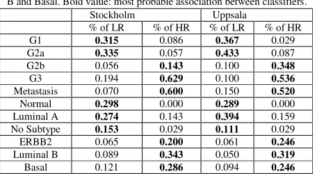
Next, we show that re-classification of grade 2 breast tumors onto genetic grade 1-like and grade 3-like subtypes [2] can be related to two genetically and clinically distinct cancer subtypes (low- and high-risk survival groups). Table III shows that survival patients’ grouping is strongly correlated with the genetic classifications of breast cancers [2], [18]. Our survival composite grouping not only discriminates low- and high- aggressive tumors by G1&G1-like versus G3-like&G3 classification, but it also establishes strong prognostic association of this classification with a grouping normal-like, luminal A and “No subtype” patients versus Basal, Luminal B and ERBB2 tumor subtypes, respectively (Table III). In the studied cohorts strong associations of defined high-risk survival groups with observed distant metastases was also found.
E. Classification on to three distinct patients’ groups
In this paragraph we extend survival grouping approach to identify gene markers that can group the patients into three distinct biological groups. We call these groups low-risk, medium-risk and high-risk. Our approach considers the patients’ frequencies according to which each patient is assigned to one of the risk groups.
[image:5.612.72.549.156.393.2]Table III. Frequency distributions of breast cancer subtypes based on composite grouping. LR = low-risk; HR = high-risk. Genetic tumor grade signature [2]: G1 = Grade1, G2a = Grade2a, G2b = Grade2b, G3 = Grade3, Metastasis [2] and intrinsic molecular signature subtypes defined by k-means clustering [18]: Normal, Luminal A, No Subtype, ERBB2, Luminal B and Basal. Bold value: most probable association between classifiers.
Stockholm Uppsala
% of LR % of HR % of LR % of HR G1 0.315 0.086 0.367 0.029 G2a 0.335 0.057 0.433 0.087
G2b 0.056 0.143 0.100 0.348
G3 0.194 0.629 0.100 0.536
Metastasis 0.070 0.600 0.150 0.520
Normal 0.298 0.000 0.289 0.000
Luminal A 0.274 0.143 0.394 0.159
No Subtype 0.153 0.029 0.111 0.029
ERBB2 0.065 0.200 0.061 0.246
Luminal B 0.089 0.343 0.050 0.319
[image:6.612.65.293.96.221.2]Basal 0.121 0.286 0.094 0.246
Table IV. Classification of breast cancer subtypes based on composite three groups design. LR = low-risk; HR = high-risk; MR = medium-risk. Other notations see in Table III.
Stockholm Uppsala
% LR % MR % HR % LR % MR % HR
G1 0.46 0.12 0.00 0.50 0.13 0.06 G2a 0.50 0.13 0.00 0.49 0.26 0.00
G2b 0.00 0.15 0.12 0.00 0.28 0.31
G3 0.00 0.47 0.82 0.01 0.33 0.63
Metastasis 0.05 0.34 0.71 0.15 0.36 0.53
Normal 0.33 0.00 0.00 0.40 0.09 0.00
Luminal A 0.27 0.24 0.09 0.43 0.27 0.08
No Subtype 0.17 0.03 0.00 0.13 0.07 0.00
ERBB2 0.04 0.24 0.14 0.01 0.14 0.11
Luminal B 0.05 0.27 0.42 0.02 0.18 0.25
Basal 0.11 0.20 0.33 0.01 0.25 0.56
frequencies are similar. Those, we assigned automatically to the medium-risk group. Their composite low-risk group frequencies vary between 50-70% (their high-risk frequencies vary between 50-30%).
Figure 5 (red lines) show the three group design in comparison to the composite two groups. Noticeably, our three groups improve patients’ high and low-risk groups in both cohorts, whereas indicate the existence of a separate medium-risk group. Table IV is the correlation of clinical characteristics versus the three groups. Evidently, there is a significant improvement in our high- and low- risk classification (Table III). The medium-risk group seems to be composed by very heterogeneous cancer patients, which can be studied in a future.
IV. DISCUSSION
We presented a novel approach to identify survival significant gene and gene pairs in genome-scale studies, which can be subsequently used as an input in reconstruction analysis of biological programs/pathways associated with aggressiveness of cancers and genetic diseases. Our 1-D and 2-D survival significant gene signatures are significantly associated with survival of breast cancer patients and simultaneously provide biologically meaningful information and novel cancer-associated gene targets. Our composite patients’ grouping method sorts all 2D data-driven pairs in terms of their synergetic P values (from lowest to highest P values) and also selects the top-level genes using our
voting-based classification algorithm. The composite patients’ grouping results are strongly correlated with current genetic classifications of breast cancers subtypes reported in [2, 18]. Strong association of our classification with metastasis events was also found.
Interestingly, many biologically essential and clinically important genes (e.g. MELK, BIRC5, ZWINT) can be found in our 335-gene signature; many genes and their products of the signature might be considered as potentially important risk-factors. Finally, we suggest that our survival composite grouping, genetic grade signature [2] and intrinsic molecular signature [18] could be used in concordant manner for reliable evaluation of aggressiveness of primary tumors and for individual prognosis of disease risks (metastases) of breast cancer patients after their surgery treatment.
REFERENCES
[1] L.J. van’t Veer et al, “Gene expression profiling predicts clinical outcome of breast cancer,” Nature, vol. 415, 2002, pp 530-536. [2] A.V. Ivshina et al, “Genetic reclassification of histologic grade
delineates new clinical subtypes of breast cancer,” Cancer Research, vol. 66, 2006, pp 10292-10301.
[3] Y. Pawitan et al, “Gene expression profiling spares early breast cancer patients from adjuvant therapy: derived and validated in two population-based cohorts,” Breast Cancer Research, vol. 7, 2005, pp R953-R964.
[4] E.T. Liu, V.A. Kuznetsov and L.D. Miller, “In the pursuit of complexity: Systems medicine in cancer biology,” Cancer Cell, vol. 9, 2006, pp 245-247.
[5] V.A. Kuznetsov, O.V. Senko, L.D. Miller and A.V. Ivshina, “Statistically Weighted Voting Analysis of Microarrays for Molecular Pattern Selection and Discovery Cancer Genotypes,” International Journal of Computer Science and Network Security, vol. 6, 2006, pp 73-83.
[6] E. Bair and R. Tibshirani, “Semi-supervised methods to predict patients survival from gene expression data,” PLOS Biology, vol. 2, 2004, pp 511-521.
[7] E. Motakis, A.V. Ivshina, V.A. Kuznetsov, “Data-driven approach to predict survival of cancer patients,” IEEE Engineering in Medicine and Biology, vol. 28, 2009, pp 58-66.
[8] D. LeBrun et al, “Predicting outcome in follicular lymphoma by using interactive gene pairs,” Clin Cancer Res., vol. 14, 2008, pp 478-487. [9] M.P. Goetz et al, “A two-gene expression ratio of homeobox 13 and
interleukin-17B receptor for prediction of recurrence and survival in women receiving adjuvant tamoxifen,” Clin Cancer Res., vol. 12, 2006, pp 2080-2087.
[10] R.D. Cox and D. Oakes, Analysis of Survival Data. Chapman and Hall, London, 1984.
[11] W.H. Press, B.P. Flannery, S.A. Teukolsky and W.T. Vetterling,
Numerical Recipes in C: The Art of Scientific Computing. Cambridge University Press, 1992.
[12] R.A. Irizarry, B.M. Bolstad, F. Collin, L.M. Cope, B. Hobbs and T.P. Speed, “Summaries of Affymetrix GeneChip probe level data,”
Nucleic Acids Research, vol. 31, 2003, e15.
[13] T.M. Loughin, “A residual bootstrap for regression parameters in proportional hazards model,” Journal of Stat and Comp Simulations, vol. 52, 1995, pp 367-384.
[14] D.R. Cox and E.J. Snell, “A general definition of residuals (with discussion),” Journal of the Royal Statistical Society, Series B, vol. 30, 1968, pp 248-265.
[15] B. Efron and R.J. Tibshirani, An Introduction to the Bootstrap. New York: Chapman and Hall, 1994.
[16] Y. Benjamini and Y. Hochberg, “Controlling the false discovery rate: a practical and powerful approach to multiple testing,” Journal of the Royal Statistical Society, Series B, 57, 1995, 289–300.
[17] Y. Benjamini and D. Yekutieli, “The control of the false discovery rate in multiple testing under dependency,” Annals of Statistics, 29, 2001, 1165–1188.
[image:6.612.65.302.269.410.2]