Abstract—Homogeneous wireless sensor networks (WSNs) are organized using identical sensor nodes, but the nature of WSNs operations results in an imbalanced workload on gateway sensor nodes which may lead to a hot-spot or routing hole problem. The routing hole problem can be considered as a natural result of the tree-based routing schemes that are widely used in WSNs, where all nodes construct a multi-hop routing tree to a centralized root, e.g., a gateway or base station. For example, sensor nodes on the routing path and closer to the base station deplete their own energy faster than other nodes, or sensor nodes with the best link state to the base station are overloaded with traffic from the rest of the network and experience a faster energy depletion rate than their peers. Routing protocols for WSNs are reliability-oriented and their use of a reliability metric to avoid unreliable links makes the routing scheme worse. However, none of these reliability oriented routing protocols explicitly uses load balancing in their routing schemes. In this paper, we present a novel, energy-wise, load balancing routing (LBR) algorithm that addresses load balancing in an energy efficient manner by maintaining a reliable set of parent nodes. This allows sensor nodes to quickly find a new parent upon parent loss due to the existing of node failure or energy hole. The proposed routing algorithm is tested using simulations and the results demonstrate that it outperforms the MultiHopLQI reliability based routing algorithm.
Index Terms—Distributed routing, Experimental evaluation, Load balancing, Network longevity, Wireless sensor Networks.
I. INTRODUCTION
A common application of wireless sensor networks (WSNs) is single base station data collection, which naturally creates a many-to-one traffic pattern from the sensing nodes to the base station. Given the limited resources of WSNs, routing protocols normally avoid lossy links at all costs. Forwarding sensor nodes with particularly optimal links and on the path to the base station are thus likely to have a heavier workload than their peers, as they are chosen to relay traffic generated by source sensor nodes.
Manuscript submitted for review July 26, 2009. The International Conference on Communications Systems and Technologies 2009 (ICCST’09), San Francisco, USA, 20-22 October 2009.
Khaled Daabaj, Mike Dixon, and Terry Koziniec are with the School of Information Technology, Murdoch University, Perth, WA 6150, Australia. (Corresponding author’s e-mail: [email protected]).
This additional load shortens the lifetime of these critical sensor nodes and leads to network partitioning [1]. This phenomenon is known as the routing hole or hot spot problem; the energy-wise load balancing scheme aims to avoid the formation of routing holes, or at least reduce the significance of the problem and thus enhance the energy conservation.
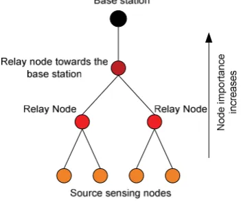
The availability of multiple routes to the sink depends on the topology of the network and its surroundings and is constrained by the radio hardware characteristics. In the best possible load balancing scenario, all sensor nodes can reach the base station directly in one hop and only send what they generate. At the opposite end of the load balancing spectrum, one particular relay or a small number thereof may be the only way for sensor nodes to reach the base station, thus forming a topological bottleneck; thereby resulting in early network partitioning. An extreme case is a linear network where only nearest-neighbor routing is possible. Figure 1 illustrates how the closer a node is to the base station, the higher its workload will be. Each relay or parent sensor node is a topological bottleneck with respect to the upstream or children sensor nodes.
Various energy-efficient paradigms and strategies have been devised to collect and route the data packets towards the base station while trying to maximize the lifetime of sensor nodes and maintain system performance and operational fidelity. According to the literature, the communication among sensor nodes consumes a large portion of the battery energy of the sensor nodes [2], some approaches focus on reducing communication power consumption, such as clustering algorithms [3], data-centric paradigms [4], and dynamic transmission power adjustment [5].
In the presence of a topological bottleneck created as a result of limitations in the routing strategy, energy efficient load balancing scheme may provide significant lifetime gains through a more efficient redistribution of the traffic workload.
Regardless of the routing strategy, the mainstream sensor nodes closer to the base station have to forward more packets than the ones at the periphery of the network. The heavier workload results in more energy consumption and the nodes closer to the base station will deplete their energy first, leading to an early loss of connectivity in the sensor network. This problem will severely reduce the effective network lifetime. To overcome this undesirable effect, a
Avoiding Routing Holes in Homogeneous
Wireless Sensor Networks
mechanism to balance the energy usage among sensor nodes is required.
Fig. 1 Sensor Network with Nearest Neighbor Routing.
The rest of the paper is organized as follows. In section II, the related work is introduced. Section III provides a brief description of the proposed routing algorithm. Section IV briefly describes performance metrics and simulations settings. The obtained results are presented in section V. Finally; Section VI ends the paper with a conclusion.
II. RELATED WORK
Tree-based routing is widely used in WSNs, where all nodes construct a multi-hop routing tree to a centralized root, e.g., gateway or base station. MintRoute [6], Directed Diffusion [4] and MultiHopLQI [7] are cost-based reliability-oriented routing protocols that are often used in WSNs. However, these cost-based routing schemes can not guarantee the maximum lifetime in the network [8]. Alternatively, maximum lifetime (lifetime-aware) routing protocols attempt to prolong network lifetime by distributing the workload among the relay nodes [9,10]. However this scheme may not have the minimum overall consumed energy [8]. This paper focuses on the balanced energy consumption model for lifetime maximization by combining elements of cost-based reliability-oriented routing schemes such as MultiHopLQI collection protocol, and maximum lifetime routing schemes such as Energy-Aware Routing (EAR) protocol [11].
However, as none of the aforementioned protocols explicitly apply a metric that considers workload balancing we have selected MultiHopLQI as a reliability-oriented cost-based routing benchmark for our simulations
.
III. ALGORITHM DESCRIPTION
A. Overview
In the parent selection process of the routing tree construction, the residual power in relay nodes and the link or channel quality between communicating nodes are the
primary factors that shape the network topology. Link or channel quality may be measured directly by most radios at the link layer, whereas residual energy can be measured and fed into the microcontroller of the sensor node at the physical layer. These parameters are used to form the cost function for the selection of the most energy efficient route. Moreover, the presence of a time constraint requires the network to favor shorter routes with a minimum number of hops in order to minimize end-to-end delay.
The routing cost function takes into account not only the current energy state of the sensor nodes and the channel state but also considers the overall distribution of the energy along the routes by means of load balancing advantages for ensuring the even distribution of traffic, which translate into more efficient energy utilization. Although the main objective of load balancing routing is the efficient utilization of WSN resources, the load balancing is an advantageous technique for evening out the distribution of loads in terms of efficient energy consumption.
Sensor nodes with the best channel qualities are considered first in the initial stages of parent selection process, while sensor nodes with the highest residual energy levels are considered afterwards. Thus, a parent is selected if it offers a reliable route, but when the traffic load increases, the remaining battery capacity of each sensor node is also accounted as the secondary metric in the parent/route selection process. The reciprocal residual energy cost function of a sensor node Si at a time is calculated to reflect the current energy status of Si. This is used to compute the cumulative route energy cost of the sensor nodes along the routing path towards the base station. Sensor nodes with low energy levels under predetermined threshold are excluded from the selected routing path to avoid sensor nodes failure due to battery outage. All routes discovered in the route searching phase are compared and the one with the least cost (the highest energy route) is selected. Sensor nodes with the highest cost (sensor nodes with residual energy levels below the predefined threshold) are banned from participating in route selection process during the route searching phase by utilizing the principle of the min-max cost function as explained in the Min-Max Battery Capacity (MMBC) routing approach [19]. From an energy cost point of view, the residual energy defines the refusal or readiness of intermediate sensor nodes to respond to route requests and forward data traffic. The maximum lifetime of a given path is determined by the weakest intermediate sensor node, which is that with the highest cost.
B. Least Cost route
The construction of the routing tree is performed in three subsequent phases: Route searching, Data transmission, and Route maintenance.
and to measure their energy and link costs from the source sensor nodes to base station. Through this message, the receiving nodes determine all routes with their costs and parent selection parameters (residual energy level, link quality information and hop count) towards the base station. The base station is assigned with a tree level or depth equal to zero, the cost parameters are also set to zero before sending the setup message.
The intermediate sensor nodes (one-hop from the base station), that can receive the route setup message from the base station, forward the route setup packets to the adjacent sensor nodes to keep them updated with a route cost towards the base station. Therefore at a sensor node Si, the route setup message is sent to an adjacent sensor node located on the routing path toward the source sensor nodes.
The adjacent sensor nodes (two-hops from the base station) forward the updated route setup message. Intermediate sensor nodes that have a higher cost compared with other peer sensor nodes (lower residual energy level and/or less link reliability) are discarded from the routing table.
The next hop sensor nodes repeat the previous steps and all information travels until it reaches the leaf source sensor nodes. At this point all nodes know their depth and the tree is fully defined.
Data transmission phase: In this stage, the source sensor nodes start to transmit data packets towards the base station through the predetermined least-cost path which was built in the route setup stage and chosen according to the parent selection parameters. In other words, the source sensor nodes send their data packets to their parents based on the forwarding parameters in the routing table. Repetitively, intermediate sensor nodes convey the data packets to the upstream parents toward the base station. This process continues until the data packets of interest reach the base station.
Route maintenance phase: Route maintenance is performed using periodic beacons to handle link dynamics and disconnection failures. Hence, the routes to all sensor nodes are kept available before any data packet transmissions occur. Source sensor nodes continue transmitting beacon packets every 15 seconds in order to sustain the routing tree and update the neighbor routing tables with forwarding nodes with the residual energy level over the threshold for all communications, and to avoid unreliable links.
IV. PERFORMANCE EVALUATION
A. Performance Metrics
Three important performance metrics are selected to analyze the performance of the proposed algorithm against MultiHopLQI routing protocol [7]:
Functional network lifetime can be obtained by calculating the average time between the commencement of the simulation and last data packet received at the base station.
Average dissipated energy is defined as the average energy consumed by the sensor node to transmit or forward data packets from the source node to the base station. This metric is used to indicate the energy efficiency level of the deployed WSN as indicated in [4,12]. The average dissipated energy can be calculated from equation 1 by taking the average for the total energy dissipated per relay sensor node. For leaf or source sensor nodes at which the data packets were originated, the energy dissipated by the receiver circuitry per bit is assigned to zero.
where,
M = the total number of operational sensor nodes.
N = the amount of data packets received.
Packet delivery ratio (PDR) is the fraction of the successfully delivered data packets to the base station divided by those generated and transmitted by sensor source nodes as in equation 2. This metric also indicates transmission success rate. The higher the packet delivery ratio, the lower the packet loss, the more efficient the routing protocol from the data delivery point of view.
B. Simulations Settings
Simulations were conducted using Matlab® with a maximum of 100 sensor nodes deployed randomly in a sensor field of 100x100 meters square with a single stationary base station. The base station was deployed on the periphery of the sensor field to increase the network depth. Each sensor node has a constant transmission range and uses a constant rate of one beacon per second for transmitting route maintenance control beacons. The maximum link layer packet size is taken from the default maximum packet transferable using TinyOS-2.x with CC2420, which is 29 bytes. Performance comparisons were conducted between the proposed load balancing scheme (LBR) and the benchmark scheme “MultiHopLQI”. To minimize the variations on routing performance from MAC layer, no energy conservation strategy is introduced in the MAC protocol. By this, the most conservative measurements are tending to be given on the advantages of
) 1 ( * 1
Re
N M
E Energy Dissipated Average
M
i
lay i
¦
==
) 2 (
Packets d Transmitte of
Number Total
Packets Delivered ly
Successful of
energy conservation routing strategy for LBR over the benchmark scheme.
V. SIMULATIONS RESULTS
In this section, the results are obtained using Matlab®-based simulations, and are analyzed with three performance metrics.
A. Network Lifetime: Figure 2 shows the time when the residual energy levels of sensor nodes drain-out and how the sensor network becomes disconnected when all the sensor nodes which can relay data packets toward the perimeter base station have died. From the figure, it can be observed that LBR performs better than MultihopLQI as the lifetimes of individual sensor nodes have been maximized. MultihopLQI protocol balances the traffic load using different paths occasionally as a direct effect of LQI values in the route selection, thereby resulting in a balanced energy consumed by few relay sensor nodes. The workload through other sensor nodes can be sub-optimal which significantly increases their residual energy dissipation in rerouting upstream data packets. Therefore, in MultihopLQI, many heavily loaded sensor nodes along the routing path die in a short period of time and the total number of sensor nodes that die is very high, while lightly loaded sensor nodes die very late.
These lightly loaded sensor node are much fewer. On the other hand, LBR conveys data packets through sensor nodes with higher residual energy levels, thus the least number of nodes are dead during the same period of time. LBR balances the energy consumption by periodically updating energy efficient routes. As the residual energy of an individual sensor node decreases to the threshold, the cost of using outgoing links from that sensor node increases.
Fig. 2 Lifespan of Individual Sensor Nodes
The network lifetime with load balancing routing has a substantial increase of approximately three times than MultiHopLQI routing. It can also be observed that the number of dead sensor nodes with load balancing routing rises gradually with time than the benchmark routing protocol. It obviously demonstrates that load balancing routing scheme can maximize the network lifetime. Since dynamic
transmission power adjustment paradigm reduced the transmission power consumption, the lifetimes of sensor nodes in variable transmission energy model could be longer than double the lifetimes of nodes in a constant transmission energy model [13,14]. Clearly, equipping sensor nodes with power control transmitters can increase lifetimes of sensor nodes. The energy consumed in processing and receiving a packet is independent of the distance between the transmitter and the receiver. Therefore, the actual increase in the lifetime depends on the energy dissipated by the transmitter amplifier, which is proportional to the distance between the transmitter and the attended receiver. Studying network lifetime with variable transmission power has been left for future work as it is out of the scope of this paper.
Figure 3 shows that the network lifetime has a deteriorating trend as the node density increases due to an abundance of control and data packets that are retransmitted throughout the network. Comparing with the benchmark scheme, the network lifetime with load balancing routing has a substantial increase of 20-30% over MultiHopLQI routing.
It can be also seen that the network lifetime with load balancing routing degrades more gracefully and it is more stable than MultiHopLQI routing protocol when the node density increases. The simulation results match with the assumption made initially that the network lifetime can be extended by transmitting aggregated data packets over energy balanced routes. The MultiHopLQI routing protocol uses its default link quality information to occasionally distribute the load over likely sub-optimal routes which is an implicit outcome of the LQI metric. Although this mechanism may not always be as efficient as the proposed load balancing algorithm, it can avoid network partitioning irregularly at an early stage.
Fig. 3 Average Network Lifetime
between different sensor nodes rapidly deplete the available energy.
B. Average Dissipated Energy: Figure 4 illustrates the relationship between the average dissipated energy during network operation and the density of the sensor field. As an overall trend it can be seen that the averaged dissipated energy by the sensor nodes in both routing algorithms has an increasing trend as the network density becomes high for the same squared sensor field size. Comparing with MultiHopLQI, LBR performs quite well where the energy consumption increases steadily with the size of the neighboring nodes. In contrast, the MultiHhopLQI dissipates more energy for the same network size and the energy dissipates considerably after escalating the node density by 50 sensor nodes. It demonstrates that LBR routing scheme outperform MultiHopLQI with the variation of the network density.
To study the influence of network densities on energy consumption, evaluations under various densities are conducted. Different scenarios with 10–100 sensor nodes were deployed arbitrarily in a fixed 100x100 meters square sensor field area, in increments to 30, 50, 70, and 100 nodes.
Figure 5 shows the change in the node’s average residual energy level after a period of data transmission. It is apparent that the network density has an impact on the individual node’s residual energy level. As an overall trend, the average remaining energy level decreases with higher density. MultiHopLQI cannot reduce the redundant data copies in the network which resulted in a high traffic load for each individual forwarding node. This makes the average remaining energy level for MultiHopLQI degrade much faster than the load balancing routing mechanism which keeps a balanced network workload towards the base station to maintain balanced energy dissipation.
Fig. 4 Average Dissipated Energy
Fig. 5 Node Residual Energy Ratio
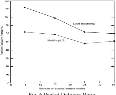
C. Packet delivery ratio: This metric is the percentage of the summation of all unique injected and aggregated packets from randomly selected source sensor nodes and received by the base station [47]. Figure 6 shows that LBR outperforms MultiHopLQI and delivers obviously a higher percentage of packet delivery rates in all load scenarios. This is due to the random selection of source nodes and the implementation of data packets aggregation. MultiHopLQI maintains a relatively steady packet delivery rate for all load scenarios. The consistent packet delivery rates for LBR in the random network show its scalability and reliability. In LBR, the average packet delivery rate is approximately 76% while in MultiHopLQI; the packet delivery rate is moderately lower by 21%.
[image:5.595.325.522.578.739.2]The random topology was simulated with an assumption that when the node transmits a packet, it has a 90% chance of being successfully delivered to the next hop or the selected parent node. This doesn’t accurately reflect the observation that some packets are skipping over the intended node in real wireless networks. In the end, the simulation results show that the packet delivery rates are much higher than the experimental results because the simulation links are based on connectivity matrix and do not consider the signal attenuation [15].
VI. CONCLUSION AND FUTURE WORK
In this paper, an energy-efficient load-balancing routing algorithm has been presented and benchmarked with the state-of-the art reliability-oriented collection protocol. The proposed algorithm incorporates the residual energy of the relay nodes with the link state in the parent selection decision to distribute the load among the sensor nodes in order to prolong the entire network lifetime. The results show that energy balance is advantageous for network lifetime extension.
Through intensive simulations in Matlab®, the feasibility of the load balancing scheme is shown by demonstrating the improved network lifetime in several deployment scenarios. Additionally, it has been observed that significant advantages can be obtained by designing and implementing a routing algorithm for WSNs with an integrated energy-wise load balancing scheme. This useful information will be used for the parent selection for the converge-cast routing tree to keep the workload balanced along the routing path.
Two extensions are suggested for future work: using substantial noise margin in parent selection to enhance stability and reliability, and utilizing the expected transmission count (EXT) metric [16-18] for reliable opportunistic data forwarding. Other improvements have been left for future work such as forwarding queue management by keeping originating data rate lower than the forwarding rate, and considering fair queuing with traffic congestion levels. This extension is an application dependent so it was kept optional to avoid algorithm complexity.
REFERENCES
[1] M. Haenggi. Energy-balancing strategies for wireless sensor networks. In IEEE International Symposium on Circuits and Systems (ISCAS'03), Bangkok, Thailand, May 2003.
[2] J. Hill, R. Szewczyk, A. Woo, S. Hollar, D. Culler, and K. Pister. System architecture directions for networked sensors. In International Conference on Architectural Support for Programming Languages and Operating Systems (ASPLOS), 2000.
[3] S. Bandyopadhyay and E. J. Coyle. “Minimizing communication costs in hierarchically-clustered networks of wireless sensors,” The International Journal of Computer and Telecommunications Networking, 44(1):1–16, 2004.
[4] C. Intanagonwiwat, R. Govindan, and D. Estrin. Directed diffusion: a scalable and robust communication paradigm for sensor networks. In Proceedings of the 6th Annual International Conference on Mobile Computing and Networking (MobiCom), pages 56–67, 2000.
[5] A. Muqattash and M. M. Krunz. A distributed transmission power control protocol for mobile ad hoc networks. IEEE Transactions on Mobile Computing, 3(2):113–128, 2004.
[6] A. Woo, T. Tong, and D. Culler. Taming the Underlying Challenges of Reliable Multihop Routing in Sensor Networks. In Proceedings of the 1st International Conference on Embedded Networked Sensor Systems (SenSys’03), Los Angeles, CA, USA, November 2003. [7] Tinyos multihoplqi collection protocol, “MultiHopLQI”.
http://www.tinyos.net/tinyos-1.x/tos/lib/MultiHopLQI/
[8] J. N. Al-Karaki and A. E. Kamal, “Routing techniques in wireless sensor networks: a survey,” IEEE [see also IEEE Personal Communications] Wireless Communications, vol. 11, no. 6, pp. 6–28, Dec. 2004.
[9] A. Sankar and Z. Liu, Maximum lifetime routing in wireless ad-hoc networks, IEEE INFOCOM 2004.
[10] J. Park and S. Sahni, Maximum Lifetime Routing in Wireless Sensor Networks, Computer & Information Science & Engineering, University of Florida, June 2, 2005.
[11] R. Shah, J. Rabaey. Energy aware routing for low energy ad hoc sensor networks. Proceedings of IEEE WCNC’02, Orlando, FL, March 2002; 350–355.
[12] A. Woo, and D. Culler, A transmission control scheme for media access in sensor networks, Proceedings of ACM MobiCom 01, Rome, Italy, July 2001, pp. 221–235.
[13] J. Chang and L. Tassiulas. Maximum lifetime routing in wireless sensor networks. IEEE/ACM Transactions on Networking, 12(4):609–619, 2004.
[14] A. Muqattash and M. M. Krunz. A distributed transmission power control protocol for mobile ad hoc networks. IEEE Transactions on Mobile Computing, 3(2):113–128, 2004.
[15] T. S. Rapport, “Wireless Communications: Principles and Practice,” Prentice Hall, 1992.
[16] D. De Couto, D. Aguayo, J. Bicket, and R. Morris. A High-Throughput Path Metric for Multi-Hop Wireless Routing. In Proceedings of the 9th Annual International Conference on Mobile Computing and Networking (MobiCom’03), San Diego, CA, USA, 2003.
[17] S. Biswas and R. Morris, Opportunistic Routing in MultiHop Wireless Networks, ACM SIGCOMM’05, Philadelphia, Pennsylvania, USA, August 2005.
[18] R. Shah, S. Wietholter, A. Wolisz, J. Rabaey. When does opportunistic routing make sense?. In the proceedings of the Third IEEE International Conference on Pervasive Computing and Communications (PerCom’05) Workshops, March 2005.
[19] C.-K. Toh, “Maximum battery life routing to support ubiquitous mobile computing in wireless ad hoc networks,” Comm. Mag., IEEE, June 2001, vol.39, issue 6, pp. 138-147.