Abstract—In the design process of complex systems, the designer is solving an optimization problem, which involves different disciplines and where all design criteria have to be optimized simultaneously. Mathematically this problem can be reduced to a vector optimization problem. The solution of this problem is not unique and is represented by a Pareto surface in the space of the objective functions. Once a Pareto solution is obtained, it may be very useful for the decision-maker to be able to perform a quick local approximation in the vicinity of this Pareto solution in order to explore its sensitivity. In this paper, a method for obtaining linear and quadratic local approximations of the Pareto surface is derived. The concept of a local quick Pareto analyser is proposed. This concept is based on a local sensitivity analysis, which provides the relation between variations of the different objective functions under constraints. A few examples are considered.
Index Terms—Pareto surface approximation, multi-objective optimization, sensitivity analysis, trade-off.
I. INTRODUCTION
In the process of designing complex systems, contributions and interactions of multiple disciplines are taken into account to achieve a consistent design. In practice, the design problem is made even more complicated because the decision maker (DM) has to consider many different and often conflicting criteria. In fact, during the optimization process, the DM often has to make compromises and look for trade-off solutions rather than a global optimum, which usually does not exist. Multi-disciplinary design optimization (MDO) has become a field of comprehensive study for the last few decades, especially since the computer power has begun to satisfy some minimal requirements to tackle this problem. MDO embodies a set of methodologies, which provide means of coordinating efforts and performing the optimization of a complex system. Two fundamental issues associated with the MDO concept are the complexity of the problem (large number of variables,
Manuscript received March 21, 2006. The research reported in this paper has been carried out within the VIVACE Integrated Project (AIP3 CT-2003-502917) which is partly sponsored by the Sixth Framework Programme of the European Community under priority 4 “Aeronautics and Space”.
S.V. Utyuzhnikov is with the School of Mechanical, Aerospace & Civil Engineering, University of Manchester, Sackville Street, P.O. Box 88, Manchester, UK, M60 1QD (e-mail: [email protected]). J. Maginot is with the Department of Aerospace Engineering, School of Engineering, Cranfield University, Cranfield, MK43 0AL, UK (e-mail: [email protected]).
M.D. Guenov is with the Department of Aerospace Engineering, School of Engineering, Cranfield University, Cranfield, MK43 0AL, UK (e-mail: [email protected]).
constraints and objectives) and the difficulty to explore the whole design space. Thus, in practice the DM would benefit from the opportunity to obtain additional information about the model without running it extensively.
Finding a solution to an MDO problem implies solving a vector optimization problem under constraints. In general, the solution of such a problem is not unique. In this respect, the existence of feasible solutions, i.e. solutions that satisfy all constraints, but cannot be optimized further without compromising at least one of the other criteria leads to the Pareto optimal concept [1]. Each Pareto point is a solution of the multi-objective optimization problem. The DM often selects the final design solution among an available Pareto set based on additional requirements that are not taken into account in the mathematical formulation of the vector optimization problem.
In spite of the existence of many numerical methods for non-linear vector optimization, there are few methods suitable for real-design industrial applications. In many applications, each design cycle includes time-consuming and expensive computations of each discipline.
In preliminary design it is important to get maximum information on a possible solution at a reasonably low computational cost. Thus, it is very desirable for the DM to be able to approximate the Pareto surface in the vicinity of a current Pareto solution and to provide its sensitivity information [2]. It would also be very useful for the DM to be able to carry out a local approximation of other optimal solutions relatively quickly without additional full-run calculations. Such an approach is based on a local sensitivity analysis (SA) providing the relation between variations of different objective functions under constraints.
Currently, only a few papers are devoted to the SA of Pareto solution in MDO [2]-[6]. They are based on the application of the gradient projection method (GPM) [7] which was first used in [3]. The SA analysis based on a local linear approximation geometrically results in finding the hyperplane tangent to the Pareto surface at some Pareto point. The quadratic approximation is based on an approximate evaluation of the local Hessian [2]. Such an approximation is based on the assumption of the local availability of some other Pareto solutions. The generation of such solutions can be done by the method developed in [8], [9]. However, this assumption may not be always valid. One of the most difficult problems in the SA is related to possible non-smoothness of the Pareto surface in the objective space and is addressed in [5], [6].
The objective of this work is to develop a method for local trade-off analysis and approximation of the Pareto surface at a differentiable Pareto solution. Linear and quadratic analytical local approximations of the Pareto front are obtained. It is
Local Approximation of Pareto Surface
shown that the linear approximation of the Pareto surface obtained in [3] determines in the objective space a local hyperplane tangent to the Pareto surface only under particular conditions. The concept of a local quick Pareto analyzer based on the local linear and quadratic approximations of the Pareto surface is suggested. It enables the DM to analyze the trade-off between different objective functions without full time-consuming optimization. While improving one objective function the DM has an opportunity to determine the trade-offs to be made on the others. In addition, it is possible to evaluate the gain of one objective function at the expense of another one.
II. MULTI-OBJECTIVE OPTIMIZATION PROBLEM An optimization problem is described in terms of a design variable vector x = (x1,x2,…,xN)T in the design space X ⊂\N.
A function f ∈ \Mevaluates the quality of a solution by
assigning it to an objective vector y =(y1,y2,…,yM)T where each
objective yi = fi(x), fi: \N→\1, i=1,…, M in the objective space
Y ⊂ \M. Thus, X is mapped onto Y by f: X→Y. A
multi-objective optimization problem can be formulated in the following form:
Minimize [ ( )]y x (2.1)
Subject to L inequality constraints
i
g ( ) 0x ≤ i = 1,...,L
(2.2) which may also include equality constraints.
A feasible design point is a point that does not violate any constraints. Therefore the feasible design space X* is defined as
the set {x | gi(x)≤ 0, i=1,…,L}. The feasible criterion (objective) space Y* is defined as the set {Y(x)| x ∈ X*}.
A design vector a (a ∈ X*) is called a Pareto optimum if, and
only if, it does not exist any b ∈ X*such that yi(b) ≤ yi(a), i =1,…, M and there exist 1 ≤ j ≤Msuch that: yi(b) < yi(a). Here and further it is supposed that all vectors are considered in the appropriate Euclidean spaces.
III. PARETO APPROXIMATION
In this section, we assume that the Pareto surface is smooth in the vicinity of the Pareto solution under study. A local approximation of the Pareto surface would allow the DM to obtain quickly both qualitative and quantitative information on the trade-off between different local Pareto optimal solutions. A constraint is said to be active at a Pareto point x* of the
design space X if a strict equality holds at this point [3]. In this
section, it is assumed that constraints that are active at a particular Pareto point remain active in its vicinity. Thus, the sensitivity predicted at the given Pareto point is valid until the set of active constraints remains unchanged [2], [3]. Without loss of generality, let us assume that the first I constraints are active and the first Q of those correspond to inequality constraints (Q ≤ I ≤ L).
Let us note the set of active constraints (2.2) as G ∈ \I. At the
given point x* of the design feasible space X* it means:
*
G(x )=0. (3.1)
Assume that G ∈ C1(\I), thenlocally the constraints can be
written in the linear form: *
J(x−x )=0
,
(3.2)
where J is the Jacobian of the active constraints set at x*: J=∇G. If all gradients of the active constraints are linearly
independent at a point, then this point is called a regular point [1]. Thus, we say that a point x*∈X* is regular if rank(J) = I.
Let us further assume that in the objective space Y the Pareto
surface is given by:
( ) 0
S y = (3.3)
and at the Pareto point y* = f (x*) function S ⊂C2(\1).
The values of the gradient of any differentiable function F at point x* under constraints are defined by the reduced gradient
formula (see, e.g., [10]):
|Sl
F F
∇ = ∇P (3.4)
where Sl is the hyperplane tangent to the feasible space X*:
{ ( ) 0}
l
S = * =
x | J x - x (3.5)
and P is projection matrix onto this hyperplane :
1
( ) .
T T −
= −
P I J JJ J (3.6)
Directional derivatives on corresponding to (3.4) in the objective space are represented by:
.
l
S
i i
dF dF d
df = d df
x
x (3.7)
The first element of the product corresponds to the reduced gradient. In the second element, dx represents the infinitesimal
change in the design vector x required to accommodate the
infinitesimal shift in the objective vector df tangent to the
Pareto surface.
The last derivative in (3.7) can be represented via the gradients in the design space X as follows. Assume that matrix P∇f, (f = (f1,f2,…,fM)T) has nf < M linearly independent
columns. It is to be noted that nf≠M. Indeed, since
( )T
df= P f∇ dx, (3.8)
nf =M would mean that for any df, in particular one where all
objectives are improved together, there would exist a dx so that
the set of active constraints remains unchanged. This contradicts the fact that the point under study is a Pareto solution. Indeed, in view of (3.3) we have
1 |
0
M i i i S
S df f
= ∂
= ∂
and it is easy to see that to move locally on the Pareto surface, dfi (i = 1,…,M) cannot be chosen independently.
Without loss of generality, let us assume further that the first nfcomponents of P∇f are linearly independent and represented
by: 1 ( ,..., ). f n f f ∇ ≡ ∇ ∇
P f P P (3.10)
Therefore, (3.8) reduces to
( )T .
df= P f∇ dx (3.11)
Now, let us write dx in the following form:
.
d
x
=
A f
d
(3.12) Then, having multiplied both sides of (3.12) by ( ∇ )TP f and
taking into account (3.11) we obtain that
( ∇ )T d =d .
P f A f f (3.13)
Hence,
1
[( )T ] .−
= ∇ ∇ ∇
A P f P f P f (3.14)
Thus, matrix A is the right-hand generalized inverse matrix to
( ∇ ) .T
P f It is possible to prove that the inverse matrix
1
[(P f∇)TP f∇]− is always non-singular because all the vectors
P∇fi, (i = 1,…, nf) are linearly independent. From the definition
of matrix A it follows that (P f∇)TA=I and T
i ∇ =fj ij
A P δ ,
where I is the unit matrix and δijis the Kronecker symbol.
Hence, the system of vectors
{ }
Ai (i=1,...,nf) creates the basis reciprocal to the basis of vectors{
P∇fj}
(j=1,...,nf). From (3.14) it follows that PA = A and dx in (3.12) belongsto the tangent plane Sl at the Pareto point.
Thus,
1
[( )T ]
d d
−
= ≡ ∇ ∇ ∇
x
A P f P f P f
f
(3.15)
and for any i≤nf :
,
i d df = i
x
A (3.16)
where A=(A A1, 2,...,Anf).Then, from (3.4), (3.7) and (3.15) it follows that for any i≤nf:
( )T T T
i i i
i
dF
F F F
df = ∇P A =A P∇ =A ∇ (3.17)
If F = fj, (nf < j ≤M), then we can obtain the sensitivity of an
objective fj along the feasible descent direction of an objective fi. Thus,
(0 , ).
j T
i j f f
i
df
f i n n j M
df =A ∇ ≤ ≤ < ≤ (3.18)
It is important to note that this formula coincides with the formula:
( , ) ( , )
( , ) ( , )
j j i j i
i i i i i
df f f f f
df f f f f
∇ ∇ ∇ ∇
= ≡
∇ ∇ ∇ ∇
P P P
P P P (3.19)
obtained in [3] if and only if either the vectors P f∇create an
orthogonal basis or nf = 1. In this case, the matrix (P f∇)TP f∇
is diagonal. In particular, these formulas always coincide in the case of two-objective optimization since nf = 1.
On the Pareto surface in the objective space the operator of the first derivative can be defined by:
.
T i i
d
df =A ∇ (3.20) By applying this operator to the first order derivative found previously, one can obtain the reduced Hessian as follows:
(
)
2
2 (0 , ).
T T T
i j i j f
i j
d F
F F i j n
df df =A ∇ A ∇ ≈A ∇ A ≤ ≤ (3.21)
Thus, the Pareto surface can be locally represented as a linear hyperplane: 1 0 f n i i i dS f df = Δ =
∑
(3.22)or a quadratic surface:
2 1 , 1
1
0 2
f f
n n
i j k
i j k
i j k
dS d S
f f f
df df df
= =
Δ + Δ Δ =
∑
∑
(3.23)where ∆f = f – f(x*).
Approximations (3.22) and (3.23) can be rewritten with respect to the trade-off relations between the objective functions as follows:
* 1
( 1, ..., ),
f
n p
p p i f
i i
df
f f f p n M
df
=
= +
∑
Δ = + (3.24)( ) *
1 , 1
1
( 1, ..., ), 2
f f
n n
p p
p p i jk j k f
i
i j k
df
f f f H f f p n M
df
= =
= +
∑
Δ +∑
Δ Δ = +(3.25) where
Quadratic approximation (3.25) with nf = M -1 is used in [3]
where the reduced Hessian matrix Hij is evaluated with a
least-squared minimization using the Pareto set generated around the original Pareto point. In an industrial situation, such evaluation can be unsuitable because it would require generating more Pareto points in the vicinity of the point under study. Instead, the local determination of the reduced Hessian using (3.21) is more accurate and is entirely based on the value of the objective and constraint gradients with respect to the independent design variables. These gradients are calculated and used during the optimization procedure; therefore the local approximations can be obtained at no extra computational cost. It is important to note that in contrast to [3] the developed approximations precisely correspond to the first three terms of the Taylor expansion in the general case.
IV. LOCAL QUICK PARETO ANALYSIS
The first order derivatives df dfp i provide us with first
order sensitivity of an objective fp along the feasible descent
direction of an objective fi when all other objectives are kept
constant. It is to be noted here that all the derivatives df dfp i
are non-positive (1 ≤ i≤nfand nf < p≤ M). Otherwise, two objectives could be locally improved which would contradict the Pareto-solution assumption.
The local approximations of the Pareto surface can be used to study the local adaptability of a Pareto solution. Since in a real-life problem it can be very computationally expensive to obtain even a single Pareto solution, local approximate solutions around a Pareto point can be obtained using either (3.24) or (3.25).
As discussed above, in the preliminary design it can be very beneficial to the DM if s/he is able to perform quick SA of the solution obtained. Using the local approximation of the Pareto surface the DM has an opportunity to perform the SA without additional full-run computations. It is also easy to obtain the information on trade-off between different objectives. Usually, the number of objectives considered in an industrial case is larger than two. In this case, the change of one objective does not fully determine the changes of the others. If the DM freezes all objectives apart from two or three, it is then possible to obtain information which is useful for understanding the trade-off between the selected objectives. The analysis of solutions around a Pareto point allows the DM to correct locally the solution with respect to additional preferences. Furthermore, the DM is able to analyze possible violations of the constraints as part of the trade-off analysis. In the design practice, the opportunity of further improvement of some objectives at the expense of local degradation of some other objectives can also be important. Representations (3.24) and (3.25) are only local approximations and there is a question on the range of Δx where the approximation is valid. In the
framework of a local analysis, giving a strict answer to this question is not possible. Nevertheless, it is possible to evaluate qualitatively the reliable range of the variation of Δx by
comparing the solutions obtained by the linear and quadratic approximations. It is reasonable to expect that the
approximations are suitable as long as the difference between the two approximations is small.
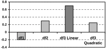
As a qualitative example, let us consider the case of an optimization problem with three objectives and assume that linear and quadratic approximations for objective f3 are
available. Assume that the DM compromises objective f2 and
improves objective f1. The local approximations (3.24) and
(3.25) provide the DM with the information on how objective f3
is affected. If the discrepancies between the linear and quadratic approximation remain relatively small in some norm, the local approximation may be considered as reliable, as shown in Figure 1.
-0.4 -0.2 0 0.2 0.4 0.6 0.8
df1 df2 df3 Linear df3
[image:4.595.322.533.244.345.2]Quadratic
Figure 1: « Reliable » local Pareto approximation
Otherwise, the local approximation is not reliable for the chosen range of variation of the design variables, as illustrated in Figure 2.
-0.4 -0.2 0 0.2 0.4 0.6 0.8
df1 df2 df3 Linear df3
Quadratic
Figure 2: « Non-reliable » local Pareto approximation
In general, the Pareto surface can be non-smooth. If the designed Pareto solution appears at a point of lack of smoothness, the approximations derived above are not formally valid. In such a case a substantial discrepancy can appear between the first and second order approximations in the vicinity of the point.
In the SA, due to a perturbation δf and the appropriate
displacement δx some constraints, which are inactive at point x*, can become either violated or active. The exact verification of the constraints validation may be time consuming. In [6], it is suggested to obtain a local linear approximation of the inactive constraints at x*to study the degree of constraint violation.
[image:4.595.322.533.434.532.2]*
( ) ( ) k , ( ),
k k j
j
dg
g g f I k L
df
= + Δ < ≤
x x (4.1)
2
* 2
2 1
( ) ( ) ( ) .
2
k k
k k j j
j j
dg d g
g g f f
df df
= + Δ + Δ
x x (4.2)
These equations can be used to verify that inactive constraints remain inactive at a new approximate Pareto point. Such verification is necessary to ensure that the assumption that the set of active constraints remains unchanged is valid and therefore that the approximation is legitimate.
V. EXAMPLE
To compare with the approach described in [3], let us consider the following multi-objective problem:
Minimise:
f=(x, y, z)T. (5.1) Subject to:
2 2 2
g( ) 1 x y z 0,
x 0, y 0, z 0.
= − − − ≤
> > > x
(5.2)
The design space and objective space coincide in this example. It is easy to see that the Pareto surface corresponds to the part of the unit sphere in the first quadrant and is represented by the following formulas:
2 2
z 1 x y ,
x 0, y 0.
= − −
> >
(5.3)
The analytical first order derivatives can be easily derived:
3
2 2 1
3
2 2 2
df dz x
df dx 1 x y
df dz y
df dy 1 x y
,
.
−
= =
− −
−
= =
− −
(5.4)
Let us derive the first order approximation using approach
[3] and the method described in this paper.
Using (3.19) and (3.6) one can obtain the first order derivatives as in [3]:
(
)
( )
( )
(
)
( )
(
)
2 2
3
2 2 2 2 2
1
2 2
3
2 2 2 2 2
2 [3]
[3]
1 x y
d xz
d y z 1 x 1 x y
1 x y
d yz
d x z 1 y 1 x y
x
y
-
-f
-f - -
-f f
-,
-. +
− −
−
+ − − −
= =
= =
(5.5)
[image:5.595.90.278.95.147.2] [image:5.595.370.498.139.237.2]Note that (5.5) are different from the exact analytical first order derivatives (5.4). They result in the approximation given in Figure 3.
Figure 3: Linear approximation [3] (unit sphere)
According to the method developed in this paper, we obtain:
1 0
0 1
y x
z z
.
⎡ ⎤
⎢ ⎥
⎢ ⎥
=
⎢ ⎥
−
⎢− ⎥
⎣ ⎦
A (5.6)
[image:5.595.378.456.288.345.2]Using (3.18) and (3.21), one can easily ensure that we obtain the exact first order and second order derivatives. The resulting linear and quadratic approximations are shown in Figure 4 and Figure 5 respectively.
Figure 4: New linear approximation (unit sphere)
Figure 5: New quadratic approximation (unit sphere)
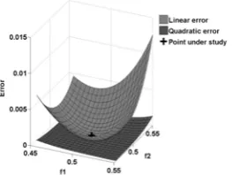
The relative error of the prediction in objective f3 is given in
[image:5.595.371.492.416.513.2] [image:5.595.371.500.546.643.2]Figure 6: Relative error in predicting f3 (unit sphere)
VI. CONCLUSION
A method for local approximation of the Pareto frontier is presented in this paper. The exact general formulas for the first and second order approximations are derived. An approach is suggested to evaluate the vicinity of the Pareto solution where the local analysis is valid. The developed concept of the local Pareto analyser allows the decision maker to perform a local analysis of the Pareto solutions and trade-offs between different objectives. Future work will concentrate on testing and application of the method to complex MDO industrial test cases.
REFERENCES
[1] K.M., Miettinen, Nonlinear Multiobjective Optimization, Kluwer Academic, Boston, 1999.
[2] S., Hernandez, “A general sensitivity analysis for unconstrained and constrained Pareto optima in Multiobjective Optimization”, AIAA-1288-CP, Proceedings of the 36th AIAA/ASME Structures
Dynamics and Materials Conference, 1995.
[3] R.V., Tappeta, and J.E., Renaud, “Interactive MultiObjective Optimization Procedure”, AIAA Paper 99-1207, April 1999.
[4] R.V., Tappeta, J.E., Renaud, A., Messac, and G.J., Sundararaj, “Interactive physical programming: trafeoff analysis and decision making in multidisciplinary optimization”, AIAA Journal, 38, Vol.5, 2000, pp. 917-926.
[5] W.H., Zhang, “Pareto sensitivity analysis in multicriteria optimization”, Finite Elements in Analysis and Design, 39, 2003, pp. 505-520. [6] W.H., Zhang, “On the Pareto optimum sensitivity analysis in multicriteria
optimization”, International Journal for Numerical Methods in Engineering, 58, 2003, pp. 955-977.
[7] J.B., Rosen, “The gradient projection method for nonlinear programming. Part I. Linear constraints”, Journal of the Society for Industrial and Applied Mathematics, 1, Vol.8, 1958, pp.181-217. [8] S.V., Utyuzhnikov, M.D., Guenov, and P., Fantini, “Numerical method
for generating the entire Pareto frontier in multiobjective optimization”, Proceedings of Eurogen’2005, Munich, September 12-14, 2005. [9] M.D., Guenov, S.V., Utyuzhnikov, and P., Fantini, “Application of the
modified physical programming method to generating the entire Pareto frontier in multiobjective optimization”, Proceedings of Eurogen’2005, Munich, September 12-14, 2005.
![Figure 3: Linear approximation [3] (unit sphere)](https://thumb-us.123doks.com/thumbv2/123dok_us/1334238.664617/5.595.371.500.546.643/figure-linear-approximation-unit-sphere.webp)