et al ., [2] proposed an algorithm to overcome this

(1)

Abstract—An improved decision-based algorithm for the restoration of gray-scale and color images that are highly corrupted by Salt-and-Pepper noise, is proposed in this paper which efficiently removes the salt and pepper noise while preserving the details. The algorithm utilizes previously processed neighboring pixel values to get better image quality than the one utilizing only the just previously processed pixel value. The proposed algorithm is faster and also produces better result than a Standard Median Filter (SMF), Adaptive Median Filters (AMF), Cascade and Recursive non-linear filters. The advantage of the proposed algorithm (PA) lies in removing only the noisy pixel either by the median value or by the mean of the previously processed neighboring pixel values. Different gray-scale and color images have been tested by using the proposed algorithm and found to produce better PSNR and SSIM values.

Index Terms—Decision-based filter, impulse noise, median filter, salt-and-pepper noise.

I. INTRODUCTION

MPULSE noise is a special type of noise which can have

many different origins. Images are often corrupted by impulse noise caused by transmission errors, faulty memory locations or timing errors in analog-to-digital conversion. Salt-and-pepper noise is one type of impulse noise which can corrupt the image, where the noisy pixels can take only the maximum and minimum values in the dynamic range. Since, linear filtering techniques are not effective in removing impulse noise, non-linear filtering techniques are widely used in the restoration process. The standard median filter (SMF) is one of the most popular non-linear filters used to remove salt-and-pepper noise due to its good denoising power and computational efficiency [3]. However, the major drawback of the SMF is that, the filter is effective only for low noise densities, and additionally, exhibits blurring if the window size is large and leads to insufficient noise suppression if the window size is small [4]. When the noise level is over 50%, the edge details of the original image will not be preserved by the median filter [2]. Nevertheless, it is important that during

Mr. Madhu S. Nair is with Rajagiri School of Computer Science, Rajagiri College of Social Sciences, Kalamassery, Kochi – 683104, Kerala, India (e-mail: [email protected], Phone: +91 94473 64158).

Prof. Dr. K. Revathy is with Department of Computer Science, University of Kerala, Karyavattom – 695581, Trivandrum, Kerala, India (e-mail: [email protected], Phone : +91 471 2416360).

Dr. Rao Tatavarti is a Research Scientist with Naval Physical & Oceanographic Laboratory (NPOL), Thrikkakara, Kochi – 682021, Kerala, India (e-mail: [email protected], Phone: +91 484 2428370).

the filtering (restoration) process the edge details have to be preserved without losing the high frequency components of the image edges [4], [5].

The ideal approach is to apply the filtering technique only to noisy pixels, without changing the uncorrupted pixel values. Non-linear filters such as Adaptive Median Filter (AMF), decision–based or switching median filters [6], [7], [8] can be used for discriminating corrupted and uncorrupted pixels, and then apply the filtering technique. Noisy pixels will be replaced by the median value and uncorrupted pixels will be left unchanged. AMF performs well at low noise densities since the corrupted pixels which are replaced by the median values are very few. At higher noise densities, window size has to be increased to get better noise removal which will lead to less correlation between corrupted pixel values and replaced median pixel values. In decision-based or switching median filter the decision is based on a pre-defined threshold value. The major drawback of this method is that defining a robust decision measure is difficult. Also these filters will not take into account the local features as a result of which details and edges may not be recovered satisfactorily, especially when the noise level is high.

Chan et al., [2] proposed an algorithm to overcome this problem, which consists of two stages. The first stage is to classify the corrupted and uncorrupted pixels by using AMF and in the second stage, regularization method is applied to the corrupted pixels to preserve edges and suppress noise. The drawback of this method is that for high impulse noise, it requires large window size of 39×39, and additionally requires complex circuitry for the implementation and determination of smoothing factor β to get good results [2]. Srinivasan and Ebenezer [1] proposed an algorithm in which the corrupted pixels are replaced by either the median pixel or neighborhood pixel by using a fixed window size of 3×3 resulting in lower processing time and good edge preservation. Although the recent technique [1] showed promising results, we discovered that a smooth transition between the pixels is lost leading to degradation in the visual quality of the image, since it only considers the left neighborhood from the last processed value. To overcome this problem we propose a new algorithm in this paper, where corrupted pixels can either be replaced by the median pixel or, the mean of the neighborhood processed pixels, which results in a smooth transition between the pixels with edge preservation and better visual quality. In addition,

Removal of Salt-and Pepper Noise in Images:

A New Decision-Based Algorithm

Madhu S. Nair, K. Revathy, and Rao Tatavarti

(2)

our proposed algorithm (PA) also uses fixed length window size of 3×3, resulting in lower processing time compared with AMF and other algorithms. It gives better Peak Signal-to-Noise Ratio (PSNR) and Structural Similarity (SSIM) index values compared to the algorithm proposed by Srinivasan and Ebenezer [1], AMF and other existing algorithms.

II. PROPOSED ALGORITHM

In most of the existing algorithms including SMF and AMF, only median values are used for the replacement of the corrupted pixels. The PA first detects the impulse noise in the image. The corrupted and uncorrupted pixels in the image are detected by checking the pixel element value against the maximum and minimum values in the window selected. The maximum and minimum values that the impulse noise takes will be in the dynamic range (0, 255) [2]. If the pixel being currently processed has a value within the minimum and maximum values in the window of processing, then it is an uncorrupted pixel and no modification is made to that pixel. If the value doesn’t lie within the range, then it is a corrupted pixel and will be replaced by either the median pixel value or by the mean of the neighborhood processed pixels (if the median itself is noisy), which will ensure a smooth transition among the pixels.

The median value itself can be noisy, especially in the case of high noise density. It is in this case, the pixel value is replaced by the mean of the neighborhood processed pixels.

⎥

⎦

⎤

⎢

⎣

⎡

4 3 2 1 4 3 2 1

Q

C

P

In the 3×3 window above, P1, P2, P3 and P4 indicates already processed pixel values, C indicates the current pixel being processed, and Q1, Q2, Q3 and Q4 indicates the pixels yet to be processed. If the median value of the above window itself is noisy, then, the current pixel value C will be replaced by the mean of the neighborhood processed pixels, that is, the mean of P1, P2, P3 and P4. The values of the pixels Q1, Q2, Q3 and Q4 will not be taken into account since they represent unprocessed pixels.

The steps of the algorithm are elucidated as follows: Step 1) Select a two dimensional window W of size 3×3. Assume that the pixel being processed is Cx,y.

Step 2) Compute - Wmin, Wmed and Wmax - the minimum, median and maximum of the pixel values in the window W respectively.

Step 3)

Case (i) If Wmin < Cx,y < Wmax, then Cx,y is an

uncorrupted pixel and its value is left unchanged. Otherwise Cx,y is a noisy pixel.

Case(ii) If Cx,y is a noisy pixel, it will be replaced by Wmed, the median value, only if Wmin < Wmed < Wmax.

Case(iii) If Wmin < Wmed < Wmax is not satisfied, Wmed itself is a noisy pixel value. In this case, Cx,y will be replaced by the mean of the neighborhood processed pixels.

Step 4) Repeat Steps 1 to 3 until all the pixels in the entire image are processed.

In the PA, the nature of the pixel being processed, that is it is corrupted or not, is checked. The value of the pixel being processed is then replaced with the corresponding value as in the Cases (i), (ii), and (iii) of Step 3. The window is then subsequently moved to form a new set of values, with the next pixel to be processed at the centre of the window. This process is repeated until the last image pixel is processed. As the most directly used color space for digital image processing, the RGB color space is chosen in our work to represent the color images. In the RGB color space, each pixel at the location (i, j) can be represented as color vector si,j = (si,jR, si,jG, si,jB), where si,jR, si,jG and si,jB are the red (R), green (G), and blue (B) components, respectively. The noisy color images are modeled by injecting the salt-and-pepper noise randomly and independently to each of these color components. That is, when a color image is being corrupted by the noise density, it means that each color component is being corrupted by p. Thus, for each pixel si,j, the corresponding pixel of the noisy image will be denoted as xi,j = (xi,jR, xi,jG, xi,jB), in which the following noise model has been used: 255 0 , , 2 1 , 2 ) ( _, = = = ⎪ ⎪ ⎩ ⎪ ⎪ ⎨ ⎧ − = x s x x for for for pp p x

f _i _j

The process of extending the noise detection algorithm to corrupted color images is straightforward. PA will be simply applied to R-, G-, and B-planes individually, and then combined to form the restored color image.

III. SIMULATION RESULTS

(3)

Structured Similarity Index (SSIM) and Image Enhancement Factor (IEF) defined as follows.

PSNR = 10*log10 (2552_/MSE)

MSE = ∑m, n [O(m, n) – R(m, n)] 2 / (M*N)

SSIM = L(O, R)*C(O, R)*S(O, R)

L(O, R) = (2µOµR+C1) / (µO2+µR2+C1)

C(O, R) = (2σOσR+C2) / (σO2+σR2+C2)

S(O, R) = (σOR+C3) / (σO σR+C3)

C1 = (K1*G)2, C2 = (K2*G)2, C3 = C2/2

G = 255; K1, K2 <<1, (K1=0.001, K2=0.002)

IEF = (∑m,n [P(m, n)–O(m, n)] 2)

/

(∑m,n [R(m, n)–O(m, n)] 2)

where, O is the original Image, R is the restored image, P is the corrupted image, MSE is the mean square error, M×N is the size of the image, L is the luminance comparison, C is the contrast comparison, S is the structure comparison, µ is the mean and σ is the standard deviation. The computation time in seconds is also computed for purposes of comparison.

Similarly, color images such as baboon.jpg and lena.jpg

of size 256×256 have been used to test the performance of the algorithm on digital color images with dynamic range of values (0, 255). Color images are corrupted by salt-and-pepper noise at different noise densities, such as low noise (30%), medium noise (60%) and high noise (90%). Then the PA is applied to the corrupted color image to remove the noise, yielding the restored color image. The performance of the color image restoration process is also quantified using PSNR, SSIM and IEF defined as follows.

PSNR = 10*log10 (2552_/MSE)

MSE = ∑m, n, x [O(m, n ,x) – R(m, n ,x)] 2 / (M*N*X)

SSIM = L(O, R)*C(O, R)*S(O, R)

L(O, R) = (2µOµR+C1) / (µO2+µR2+C1)

C(O, R) = (2σOσR+C2) / (σO2+σR2+C2)

S(O, R) = (σOR+C3) / (σO σR+C3)

C1 = (K1*G)2, C2 = (K2*G)2, C3 = C2/2

G = 255; K1, K2 <<1, (K1=0.001, K2=0.002)

IEF = (∑m, n, x [P(m, n, x)–O(m, n, x)] 2)

/

(∑m, n, x [R(m, n, x)–

O(m, n, x)] 2₎

Tables I, II and III show the performance results of the various filters, on the gray-scale images lena.tif and

cameraman.tif, at low (30%), medium (60%) and high noise (90%) densities, respectively. Tables IV, V and VI show the performance results of the various filters, on the color images

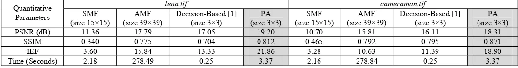
lena.jpg and baboon.jpg, at low (30%), medium (60%) and high noise (90%) densities, respectively. The results of PA (shaded in the Tables) indicate better PSNR, SSIM and IEF

values compared to SMF, AMF and the decision-based filter [1]. Although the computation time is more than decision based filter [1] and SMF, it is far better than AMF which requires 39×39 window size to get better results for high density noise. The PA uses a fixed 3×3 window size for the restoration process, which makes it faster. To calculate the computation time, MATLAB 7.0.1 on an Intel PC with 2.67GHz processor and 512 MB RAM has been used. The substantial increase in the IEF values for the PA, shown in Tables I - VI highlights the importance of our method for image restoration process.

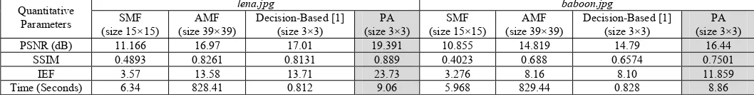
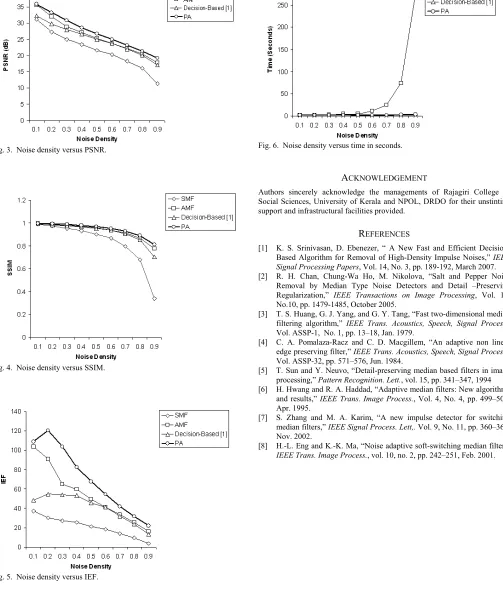
Fig.1 - 2 shows the original image, corrupted image and restored images obtained by the various filters such as, (i) SMF, which uses 5×5, 7×7, and 15×15 window size for low, medium and high noise densities respectively, (ii) AMF [2] which uses 7×7, 13×13 and 39×39 window size for low, medium and high noise densities respectively, (iii) decision-based [1] filter which uses a small fixed size 3×3 window and (iv) our PA which also uses a small fixed size 3×3 window. Figs. 3-6 show the comparison of different filters, performed on lena.tif gray-scale image at various noise densities, in terms of PSNR, SSIM, IEF and computation time. Depending on the noise density, window size varies from 3×3 to 15×15 for SMF and window size varies from 7×7 to 39×39 for AMF [2], to yield better result. For all level of noise densities decision-based filter [1] and PA use fixed size window of 3×3.

IV. CONCLUSION

In this paper, a new algorithm (PA) is proposed which gives better performance in comparison with SMF, AMF and other existing noise removal algorithms in terms of PSNR, SSIM and IEF. The proposed algorithm is faster since it uses a small window of size 3×3. In addition, it affects a smooth transition between the pixel values by utilizing the correlation between neighboring processed pixels while preserving edge details thus leading to better edge preservation.

(4)

[image:4.612.40.571.668.738.2]

(a) (b) (c) (d) (e) (f)

Fig. 1. Restoration results of different filters on gray-scale images. Columns show (a) Original Image, (b) Noisy Image, (c) SMF output, (d) AMF output, (e) Decision-Based filter [1] output, and column (f) shows the output of our PA. Rows 1, 2 and 3 shows the lena.tif image corrupted with 30%, 60%, and 90% noise respectively. Rows 4, 5 and 6 shows the cameraman.tif image corrupted with 30%, 60%, and 90% noise respectively. A comparison of images in column (b) with those in column (f) demonstrates the improved visual quality of the corrupted images.

TABLE I

PSNR, SSIM, IEF AND COMPUTATION TIME FOR VARIOUS FILTERS FOR lena.tif AND cameraman.tifIMAGES (GRAY-SCALE) AT LOW NOISE DENSITY (30%)

lena.tif cameraman.tif

Quantitative

Parameters SMF (size 5×5)

AMF (size 7×7)

Decision-Based [1] (size 3×3)

PA (size 3×3)

SMF (size 5×5)

AMF (size 7×7)

PA (size 3×3)

PSNR (dB) 24.98 28.76 27.96 30.79 21.38 25.58 23.96 27.08

SSIM 0.953 0.980 0.976 0.988 0.939 0.977 0.966 0.983

IEF 27.20 64.93 54.04 103.64 12.76 33.54 23.09 47.39

Time (Seconds) 0.26 2.32 0.27 1.77 0.26 2.32 0.27 1.75

TABLE II

PSNR, SSIM, IEF AND COMPUTATION TIME FOR VARIOUS FILTERS FOR lena.tifAND cameraman.tifIMAGES (GRAY-SCALE) AT MEDIUM NOISE DENSITY (60%)

Quantitative

AMF (size 13×13)

PA (size 3×3)

SMF (size 7×7)

AMF (size 13×13)

PA (size 3×3)

PSNR (dB) 20.27 23.74 23.73 24.95 17.55 20.73 20.93 22.29

SSIM 0.866 0.939 0.937 0.952 0.858 0.931 0.933 0.950

IEF 18.51 41.22 41.09 54.37 10.52 21.91 22.89 31.34

Time (Seconds) 0.51 11.51 0.25 1.86 0.51 11.35 0.25 1.86

TABLE III

PSNR, SSIM, IEF AND COMPUTATION TIME FOR VARIOUS FILTERS FOR lena.tifAND cameraman.tifIMAGES (GRAY-SCALE) AT HIGH NOISE DENSITY (90%)

Quantitative

Parameters SMF

(size 15×15)

AMF (size 39×39)

PA (size 3×3)

SMF (size 15×15)

AMF (size 39×39)

PA (size 3×3)

PSNR (dB) 11.36 17.79 17.05 19.20 10.70 15.81 16.11 18.31

SSIM 0.340 0.775 0.704 0.812 0.465 0.792 0.795 0.871

IEF 3.60 15.84 13.33 21.86 3.28 10.63 11.39 18.90

(5)

[image:5.612.41.570.673.741.2]

(a) (b) (c) (d) (e) (f)

Fig. 2. Restoration results of different filters on color images. Columns show (a) Original Image, (b) Noisy Image, (c) SMF output, (d) AMF output, (e) Decision-Based filter [1] output, and column (f) shows the output of our PA. Rows 1, 2 and 3 shows the lena.jpg image corrupted with 30%, 60%, and 90% noise respectively. Rows 4, 5 and 6 shows the baboon.jpg image corrupted with 30%, 60%, and 90% noise respectively. A comparison of images in column (b) with those in column (f) demonstrates the improved visual quality of the corrupted images.

TABLE IV

PSNR, SSIM, IEF AND COMPUTATION TIME FOR VARIOUS FILTERS FOR lena.jpg AND baboon.jpgIMAGES (COLOR) AT LOW NOISE DENSITY (30%)

lena.jpg baboon.jpg

Quantitative

AMF (size 7×7)

PA (size 3×3)

SMF (size 5×5)

AMF (size 7×7)

PA (size 3×3)

PSNR (dB) 23.331 27.07 26.203 29.72 18.65 21.66 19.06 23.33

SSIM 0.9568 0.9817 0.9775 0.99 0.8526 0.9293 0.8677 0.9513

IEF 19.63 46.43 38.02 85.42 6.56 13.11 7.203 19.27

Time (Seconds) 0.609 5.63 0.672 4.68 0.734 6.61 0.875 5.02

TABLE V

PSNR, SSIM, IEF AND COMPUTATION TIME FOR VARIOUS FILTERS FOR lena.jpg AND baboon.jpgIMAGES (COLOR)AT MEDIUM NOISE DENSITY (60%)

Quantitative

AMF (size 13×13)

PA (size 3×3)

SMF (size 7×7)

AMF (size 13×13)

PA (size 3×3)

PSNR (dB) 18.905 22.35 22.774 24.31 16.612 18.41 17.269 19.162

SSIM 0.8854 0.9467 0.9506 0.9651 0.7772 0.8541 0.8055 0.8724

IEF 14.14 31.25 34.45 48.97 8.244 12.49 9.594 14.84

Time (Seconds) 1.26 30.31 0.672 5.05 1.453 33.813 0.906 5.187

TABLE VI

PSNR, SSIM, IEF AND COMPUTATION TIME FOR VARIOUS FILTERS FOR lena.jpg AND baboon.jpgIMAGES (COLOR) AT HIGH NOISE DENSITY (90%)

Quantitative

Parameters SMF

(size 15×15)

AMF (size 39×39)

PA (size 3×3)

SMF (size 15×15)

AMF (size 39×39)

PA (size 3×3)

PSNR (dB) 11.166 16.97 17.01 19.391 10.855 14.819 14.79 16.44

SSIM 0.4893 0.8261 0.8131 0.889 0.4023 0.688 0.6574 0.7501

IEF 3.57 13.58 13.71 23.73 3.276 8.16 8.10 11.859

(6)

[image:6.612.319.551.64.228.2]

Fig. 3. Noise density versus PSNR.

[image:6.612.56.293.78.231.2]

Fig. 4. Noise density versus SSIM.

Fig. 5. Noise density versus IEF.

Fig. 6. Noise density versus time in seconds.

ACKNOWLEDGEMENT

Authors sincerely acknowledge the managements of Rajagiri College of Social Sciences, University of Kerala and NPOL, DRDO for their unstinting support and infrastructural facilities provided.

REFERENCES

[1] K. S. Srinivasan, D. Ebenezer, “ A New Fast and Efficient Decision-Based Algorithm for Removal of High-Density Impulse Noises,” IEEE Signal Processing Papers, Vol. 14, No. 3, pp. 189-192, March 2007. [2] R. H. Chan, Chung-Wa Ho, M. Nikolova, “Salt and Pepper Noise

Removal by Median Type Noise Detectors and Detail –Preserving Regularization,” IEEE Transactions on Image Processing, Vol. 14, No.10, pp. 1479-1485, October 2005.

[3] T. S. Huang, G. J. Yang, and G. Y. Tang, “Fast two-dimensional median filtering algorithm,” IEEE Trans. Acoustics, Speech, Signal Process., Vol. ASSP-1, No. 1, pp. 13–18, Jan. 1979.

[4] C. A. Pomalaza-Racz and C. D. Macgillem, “An adaptive non linear edge preserving filter,” IEEE Trans. Acoustics, Speech, Signal Process., Vol. ASSP-32, pp. 571–576, Jun. 1984.

[5] T. Sun and Y. Neuvo, “Detail-preserving median based filters in image processing,” Pattern Recognition. Lett., vol. 15, pp. 341–347, 1994 [6] H. Hwang and R. A. Haddad, “Adaptive median filters: New algorithms

and results,” IEEE Trans. Image Process., Vol. 4, No. 4, pp. 499–502, Apr. 1995.

[7] S. Zhang and M. A. Karim, “A new impulse detector for switching median filters,” IEEE Signal Process. Lett,. Vol. 9, No. 11, pp. 360–363, Nov. 2002.

[8] H.-L. Eng and K.-K. Ma, “Noise adaptive soft-switching median filter,”

[image:6.612.55.558.91.687.2]