Learning Discourse Relations with Active Data Selection

(1)

Learning Discourse Relations with Active D a t a Selection

T a d a s h i N o m o t o *

N a t i o n a l I n s t i t u t e of J a p a n e s e L i t e r a t u r e 1-16-10 Y u t a k a S h i n a g a w a

T o k y o 142-8585 J a p a n n o m o t o @ n i j 1. a c . j p

Y u j i M a t s u m o t o

N a r a I n s t i t u t e of Science a n d T e c h n o l o g y 8916-5 T a k a y a m a I k o m a N a r a

630-0101 J a p a n

matsu@is, aist-nara, ac.

jp

A b s t r a c t

The paper presents a new approach to identifying discourse relations, which makes use of a particular sampling m e t h o d called committee- based sampling (CBS). In the committee-based sampling, multiple learning models are generated to measure the utility of an input example in classification; if it is judged as not useful, then the example will be ignored. The m e t h o d has the effect of reducing the a m o u n t of data required for training. In the paper, we extend CBS for decision tree classifiers. W i t h an additional extension called error feedback, it is found that the m e t h o d achieves an increased accuracy as well as a substantial reduction in the a m o u n t of d a t a for training classifiers.

1 I n t r o d u c t i o n

The success of corpus-based approaches to discourse ultimately depends on whether one is able to acquire a large volume of d a t a annotated for discourse-level information. However, to acquire merely a few hundred texts annotated for discourse information is often impossible due to the enormity of the h a m a n labor required.

This paper presents a novel m e t h o d for reducing the amount of data for training a decision tree classifier, while not compromising the accuracy. While there has been some work explor- ing the use of machine leaning techniques for discourse and dialogue (Marcu, 1997; Samuel et al., 1998), to our knowledge, no computational research on discourse or dialogue so far has ad- dressed the problem of reducing or minimizing the amount of data for training a learning algorithm.

* The work reported here was conducted while the first author was with Advanced Research Lab., Hitachi Ltd, 2520 Hatoyama Saitama 350-0395 Japan.

A particular m e t h o d proposed here is built on the committee-based sampling, initially proposed for probabilistic classifiers by Dagan and Engelson (1995), where an example is selected from the corpus according to its utility in im- proving statistics. We extend the m e t h o d for decision tree classifiers using a statistical technique called bootstrapping (Cohen, 1995). W i t h an additional extension, which we call error .feedback, it is found that the m e t h o d achieves an increased accuracy as well as a significant reduction of training data. The m e t h o d proposed here should be of use in domains other t h a n discourse, where a decision tree strategy is found applicable.

2 T a g g i n g a c o r p u s w i t h d i s c o u r s e r e l a t i o n s

In tagging a corpus, we adopted Ichikawa (1990)'s scheme for organizing discourse relations (Table 1). The advantage of Ichikawa (1990)'s scheme is that it directly associates discourse relations with explicit surface cues (eg. sentential connectives), so it is possible for the coder to determine a discourse relation by figur- ing a most natural cue that goes with a sentence he/she is working on. Another feature is that, unlike Rhetorical Structure Theory (Mann and Thompson, 1987), the scheme assumes a discourse relation to be a local one, which is defined strictly over two consecutive sentences. 1 We expected that these features would make a tagging task less laborious for a h u m a n coder t h a n it would be with RST. Further, our earlier study indicated a very low agreement rate with

1This does not mean to say that all of the discourse

relations are local. There could be some relations that

involve sentences separated far apart. However we did

not consider non-local relations, as our preliminary study

(2)

Table 1: Ichikawa (1990)'s taxonomy of discourse relations. The first column indicates major classes and the second subclasses. The third column lists some examples associated with each subclass. Note that the EXPANDING subclass has no examples in it. This is because no explicit cue is used to mark the relationship.

LOGICAL

SEQUENCE

ELABORATION

CONSEQUENTIAL ANTITHESIS ADDITIVE CONTRAST INITIATION APPOSITIVE COMPLEMENTARY EXPANDING

dakara therefore, shitagatte thus shikashi but, daga but

soshite and, tsuigi-ni next ipp6 in contrast, soretomo or

tokorode to change the subject, sonouchi in the meantime

tatoeba

.for example, y6suruni in other words nazenara because, chinamini incidentally NONE

RST (~ = 0.43; three coders); especially for a casual coder, RST turned out to be a quite difficult guideline to follow.

In Ichikawa (1990), discourse relations are or- ganized into three major classes: the first class includes logical (or strongly semantic) relationships where one sentence is a logical conse- quence or contradiction of another; the second class consists of sequential relationships where two semantically independent sentences are jux- taposed; the third class includes elaboration- type relationships where one of the sentences is semantically subordinate to the other.

In constructing a tagged corpus, we asked coders not to identify abstract discourse relations such as LOGICAL, SEQUENCE and ELAB- ORATION, but to choose from a list of pre- determined connective expressions. We expected that the coder would be able to identify a discourse relation with far less effort when working with eXplicit cues t h a n when working with abstract Concepts of discourse relations. Moreover, since 93% of sentences considered for labeling in the corpus did not contain pre- determined relation cues, the annotation task was in effect one of guessing a possible connective cue that m'ay go with a sentence. The advantage of using explicit cues to identify discourse relations is that even if one has little or no background in linguistics, he or she may be able to assign a discourse relation to a sentence by just asking him/herself whether the associated cue fits well with the sentence. In addition, in order to make the usage of cues clear and un- ambiguous, the annotation instruction carried a set of examples for each of the cues. Fur-

ther, we developed an emacs-based software aid which guides the coder to work through a corpus and also is capable of prohibiting the coder from making moves inconsistent with the tagging instruction.

As it turned out, however, Ichikawa's scheme, using subclass relation types, did not improve agreement (~ = 0.33, three coders). So, we modified the relation taxonomy so that it contains just two major classes, SEQUENCE and ELABORATION, (LOGICAL relationships being subsumed under the SEQUENCE class) and as- sumed that a lexical cue marks a major class to which it belongs. The modification successfully raised the ~ score to 0.70. Collapsing LOGICAL and SEQUENCE classes may be justified by not- ing that b o t h types of relationships have to do with relating two semantically independent sentences, a property not shared by relations of the elaboration type.

3 Learning w i t h A c t i v e D a t a

Selection

3.1 Committee-based Sampling

(3)

tributions of model parameters and measuring how much the member models disagree in classifying the example. The rationale for this is: disagreement among models over the class of an example would suggest that the example affects some parameters sensitive to classification, and furthermore estimates of affected parameters are far from their true values. Since models are generated randomly from posterior distributions of model parameters, their disagreement on an example's class implies a large variance in estimates of parameters, which in t u r n indicates that the statistics of parameters involved are insufficient and hence its inclusion in the training corpus (so as to improve the statistics of relevant parameters).

For each example it encounters, CBS goes through the following steps to decide whether to select the example for labeling.

1. Draw k models (committee members) randomly from the probability distribution P ( M ] S) of models M given the statistics S of a training corpus.

2. Classify an input example by each of the committee members and measure how much they disagree on classification. 3. Make a biased r a n d o m decision as to

whether or not to select the example for labeling. This would make a highly disagreed-upon example more likely to be selected.

As an illustration of how this might work, consider a problem of tagging words with parts of speech, using a Hidden Markov Model (HMM). A (bigram) HMM tagger is typically given as:

n

T(Wl . . . Wn) = argmax ~ P(wi I ti)P(ti+l I ti)

t~ ...~ ~__~

where w l . . . w n is a sequence of input words, and t l . . . t n is a sequence of tags. For a sequence of input words w l . . . w n , a sequence of corresponding tags T ( w l . . . w n ) is one that maxi- mizes the probability of reaching tn from tl via ti (1 < i < n) and generating W l . . . w n along with it. Probabilities P(wi I ti) and P(ti+l I ti) are called model parameters of an HMM tagger. In Dagan and Engelson (1995), P ( M I S)

is given as the posterior multinomial distribution P ( a l = a l , . . . , a n = an J S), where ai is a model parameter and ai represents one of the possible values. P ( a l = a l , . . . , a n = an I S) represents the proportion of the times that each parameter oq takes a/, given the statistics S derived from a corpus. (Note that ~ P ( a i = ai I S) = 1.) For instance, consider a task of randomly drawing a word with replacement from a corpus consisting of 100 different words ( w l , . . . , Wl00). After 10 trials, you might have outcomes like wl = 3, w2 = 1 , . . . , w55 = 2 , . . . , w 7 1 = 3 , . . . , w 7 6 = 1 , . . . , w l 0 0 = 0: i.e., Wl was drawn three times, w2 was drawn once, w55 was drawn twice, etc. If you try another 10 times, you might get different results. A multinomial distribution tells you how likely you get a particular sequence of word occurrences. Da- gan and Engelson (1995)'s idea is to assume the distribution P ( a l = a l , . . . , a n = an I S) as a set of binomial distributions, each corresponding to one of its parameters. An arbitrary HMM model is then constructed by randomly drawing a value ai from a binomial distribution for a parameter ai, which is approximated by a normal distribution. Given k such models (committee members) from the multinomial distribution, we ask each of t h e m to classify an input example. We decide whether to select the example for labeling based on how much the committee members disagree in classifying that example. Dagan and Engelson (1995) in- troduces the notion of vote entropy to quantify disagreements among members. T h o u g h one could use the kappa statistic (Siegel and Castel- lan, 1988) or other disagreement measures such as the a statistic (Krippendorff, 1980) instead of the vote entropy, in our implementation of CBS, we decided to use the vote entropy, for the lack of reason to choose one statistic over another. A precise formulation of the vote entropy is as follows:

v(e, e) log V(c, e)

V ( e ) = - k

C

(4)

based on

V(e).

g

Pselect(e)

= log

k V(e)

g here is called the

entropy gain

and is used to determine the number of times an example is selected; a grea~ter g would increase the number of examples selected for tagging. Engelson and Dagan (1996) investigated several plausible approaches to the selection function but were un- able to find significant differences among them. At the beginning of the section, we mentioned some properties of 'useful' examples. A useful example is one which contributes to reducing variance in parameter values and also affects classification. By randomly generating multiple models and measuring a disagreement among them, one would be able to tell whether an example is useful in the sense above; if there were a large disagreement, then one would know that the example is relevant to classification and also is associated with parameters with a large variance and thus with insufficient statistics.

In the following section, we investigate how we might extend CBS for use in decision tree classifiers.

3.2 D e c i s i o n T r e e Classifiers

Since it is difficult, if not impossible, to express the model distribution of decision tree classifiers in terms of the multinomial distribution, we turn to the bootstrap sampling method to obtain

P(M [ S).

The bootstrap sampling method provides a way for artificially establish- ing a sampling distribution for a statistic, when the distribution is not known (Cohen, 1995). For us, a relevant statistic would be the posterior probability that a given decision tree may occur, given the training corpus.

Bootstrap Sampling Procedure

Repeat i = 1. ,. K times:

1. Draw a bootstrap pseudosample S~ of size N from S by sampling with replacement as follows:

Repeat N times: select a member of S at random ai~d add it to S~.

2. Build a decision tree model M from S~. Add M to Ss.

S is a small Set of samples drawn from the tagged corpus. Repeating the procedure 100

times would give 100 decision tree models, each corresponding to some S~ derived from the sample set S. Note that the bootstrap procedure allows a datum in the original sample to be selected more than once.

Given a sampling distribution of decision tree models, a committee can be formed by randomly selecting k models from Ss. Of course, there are some other approaches to constructing a committee for decision tree classifiers (Di- etterich, 1998). One such, known as

random-

ization,

is to use a single decision tree and randomly choose a path at each attribute test. Re- peating the process k times for each input example produces k models.

3.2.1

Features

In the following, we describe a set of features used to characterize a sentence. As a conven- tion, we refer to a current sentence as 'B' and the preceding sentence as 'A'.

<LocSen> defines the location of a sentence by:

#s(x)

# S ( Last..S entence)

' # S ( X ) ' denotes an ordinal number indicating the position of a sentence X in a text,

i.e.,

#S(kth_sentence) = k, (k >_ 0). 'Last_Sentence' refers to the last sentence in a text. LocSen takes a continuous value between 0 and 1. A text-initial sentence takes 0, and a text-final sentence 1.

<LocPar> is defined similarly to D i s t P a r . It records information on the location of a paragraph in which a sentence X occurs.

#Par(X)

#Last.Paragraph

'#Par(X)'

denotes an ordinal number indicating the position of a paragraph containing X. '#Last_Paragraph' is the position of the last paragraph in a text, represented by the ordinal number.

<LocWithinPax> records information on the location of a sentence X within a paragraph in which it appears.

(5)

'Par_Init_Sen' refers to the initial sentence of a p a r a g r a p h in which X occurs, ' L e n g t h ( P a r ( X ) ) ' denotes the number of sentences t h a t occur in t h a t paragraph. LocW:i.thinPar takes continuous values ranging from 0 to 1. A p a r a g r a p h initial sentence would have 0 and a p a r a g r a p h final sentence 1.

<LenText> the length of a text, measured in Japanese characters.

the length of A in Japanese char-

<LenSenA>

acters.

acters.

the length of B in Japanese char-

<Sire> encodes the lexical similarity b e t w e e n A and B, based on an information-retrieval measure known as

t f . idf

(Salton and McGill, 1983). 2 One i m p o r t a n t feature here is t h a t we defined similarity based on (Japanese) characters rather t h a n on words: in practice, we broke up nominals from relevant sentences into simple alphabetical characters (including graphemes) and used t h e m to measure similarity b e t w e e n the sentences. (Thus in our setup

xi

in foot- note 2 corresponds to one character, and not to one whole word.) We did this to deal with abbreviations and rewordings, which we found quite frequent in the corpus.

<Cue> takes a discrete value 'y' or 'n'. The cue feature is intended to exploit surface cues most relevant for distinguishing between the SE- QUENCE and ELABORATION relations. The fea-

2For a w o r d j in a sentence Si (j E Si), its weight wij

is defined by:

N

w# = tf~j • log ~ -

df~

is the number of sentences in the text which have an occurrence of a word j. N is the total number of sentences in the text. The

tf.idf

metric has the property of favoring high frequency words with local distribution. For a pair of sentences .,~ = (xl .... ) and Y = (yx,...), where x and y are words, we define the lexical similarity between X and Y by:

t

2 E w(xi)w(y~)

S I M ( . X , Y ) = t i=x t

E

i = 1 i = 1

where w(xi) represents a t~idf weight assigned to t h e

t e r m xi. T h e m e a s u r e is known as t h e Dice coefficient

(Salton a n d McGill, 1983)

ture takes 'y' if a sentence contains one or more cues relevant to distinguishing b e t w e e n the two relation types. We considered up to 5 word n-grams found in the training corpus. O u t of these, those whose

INFOx

values are below a particular threshold are included in the set of

c u e s . 3 A n d if a sentence contains one of the

cues in the set, it is marked 'y', and 'n' otherwise. T h e cutoff is determined in such a way as to minimize

INFOcue(T),

where T is a set of sentences (represented with features) in the training corpus. We had the total of 90 cue expressions. Note t h a t using a single binary feature for cues alleviates the d a t a sparseness problem; t h o u g h some of the cues m a y have low fre- quencies, t h e y will be aggregated to form a single cue category with a sufficient n u m b e r of instances. In the training corpus, which contained 5221 sentences, 1914 sentences are m a r k e d 'y' and 3307 are marked 'n' with the cutoff at 0.85, which is found to minimize the e n t r o p y of the distribution of relation types. It is interesting to note t h a t the entropy s t r a t e g y was able to pick up cues which could be linguistically m o t i v a t e d (Table 2). In contrast to Samuel et al. (1998), we did not consider relation cues r e p o r t e d in the linguistics literature, since t h e y would be useless unless t h e y contribute to reducing the cue entropy. T h e y m a y b e linguistically 'right' cues, b u t their utility in the machine learning context is not known.

< P r e v R e l > makes available information a b o u t a relation t y p e of the preceding sentence. It has two values, E L A for the elaboration relation, and SEQ for the sequence relation.

In the Japanese linguistics literature, there is a popular theory that sentence endings are relevant for identifying semantic relations among 3INFOx (T) m e a s u r e s t h e e n t r o p y of t h e d i s t r i b u t i o n of classes in a set T w i t h respect to a feature X . W e define INFOx j u s t as given in Q u i n l a n (1993):

xNFOx(T) = x xNFo(T,)

i = 1

Ti represents a p a r t i t i o n of T corresponding to one of

t h e values for X . INFO(T) is defined as follows:

k

INFO(T) = ~ freq(Cj, T) freq(Cj, T)

- ~ i . ~ ] x log s ] T I

j = l

(6)

I

Table 2: Some of the 'linguistically interesting' cues identified by the entropy strategy. mata on the other hand, dSjini at the same time, ippou in contrast, sarani in addition, mo topic marker, ni-tsuite-wa regarding, tameda the reason is that, kekka as the result ga-nerai the goal is that

sentences. Some of the sentence endings are inflectional categories of verbs such as PAST/NON- PAST, INTERROGATIVE, and also morpholog- ical categories :like nouns and particles (eg. question-markers). Based on Ichikawa (1990), we defined six types of sentence-ending cues and marked a sentence according to whether it contains a part.icular type of cue. Included in the set are inflectional forms of the verb and the verbal adjec~tive, PAST/NON-PAST, morpho- logical categories such as COPULA, and NOUN, parentheses (quotation markers), and sentence- final particles such as -ka. We use the following two attributes to encode information about sentence-ending cues.

<EndCueh> records information about a sentence-ending form of the preceding sentence. It takes a discrete value from 0 to 6, with 0 indicating the absence in the sentence of relevant cues.

<EadCueB> Sa~me as above except that this feature is concerned with a sentence-ending form of the current sentence, i.e. the 'B' sentence.

Finally, we have two classes, ELABORATION and SEQUENCE.

4 E v a l u a t i o n

To evaluate our method, we carried out experiments, using a corpus of news articles from a Japanese economics daily (Nihon-Keizai- Shimbun-Sha, 1995). The corpus had 477 articles, randomly selected from issues that were published durilig the year. Each sentence in the articles was tagged with one of the discourse relations at the subclass level (i.e. CONSEQUEN- TIAL, ANTITHESIS, etc.). However, in evaluation experiments, we translated a subclass relation into a corresponding major class relation (SE- QUENCE/ELABORATION) for reasons discussed earlier. Furthermore , we explicitly asked coders not to tag a paragraph initial sentence for a discourse relation, for we found that coders rarely agree on their :classifications. Paragraph-initial

sentences were dropped ffrom the evaluation corpus. This had left us with 5221 sentences, of which 56% are labeled as SEQUENCE and 44% ELABORATION.

To find out effects of the committee-based sampling m e t h o d (CBS), we ran the C4.5 (Re- lease 5) decision tree algorithm with CBS turned on and off (Quinlan, 1993) and measured the performance by the 10-fold cross validation, in which the corpus is divided evenly into 10 blocks of data and 9 blocks are used for training and the remaining one block is held out for testing. On each validation fold, CBS starts with a set of about 512 samples from the set of training blocks and sequentially examines samples from the rest of the training set for possible labeling. If a sample is selected, then a decision tree will be trained on the sample to- gether with the data acquired so far, and tested on the held-out data. Performance scores (error rates) are averaged over 10 folds to give a s u m m a r y figure for a particular learning strategy. T h r o u g h o u t the experiments, we assume that k = 10 and g = 1, i.e., 10 committee members and the entropy gain of 1. Figure 1 shows the result of using CBS for a decision tree. T h o u g h the performance fluctuates erratically, we see a general tendency t h a t the CBS m e t h o d fares better t h a n a decision tree classifier alone. In fact differences between C4.5/CBS and C4.5 alone proved statistically significant (t = 7.06, df = 90, p < .01).

(7)

Figure 1: Effects of CBS on the decision tree learning. Each point in the scatterplots represents a s u m m a r y figure,

i.e.

the average of figures obtained for a given x in 10-fold cross validation trials. The

x-axis

represents the amount of training data, and the y-axis the error rate. The error rate is the proportion of the misclassified instances to the total number of instances.

47.5

4 7

,46.5

46

45.5

45

44.5

44

43.5

43 0

@ o

o o O @ ~ o

@ @ o o

@ @@~ @ o

@ O O O :

@ @

+ O @ 0 O

"¢+ $ O : O +

o + o

@ o o : o 0

o +%+ + % > + ~+ o

+ + +++ +~ + ~ + o ~ *+

+ + + + ++ ~ + ¢ 0 + + +

.p + + +

+ _{~ + + +} ₊ O a r + +

+ + O@

4- 4-

+

I I I

200 400 600

Training Data

I

STD C4.5 CBS+C4.5 +

O @

o

o @ o o _@

o _o o o o

o ¢ o @ O

-I-k++ +

+ + +++ ++++

÷ +

+ I

8OO

0

1000

a drastic restructuring of a decision tree. In the face of this, we made a small change to the way CBS works. The idea, which we call a

sampling

with error feedback,

is to remove harmful examples from the training data and only use those with positive effects on performance. It forces the sampling mechanism to return to

status quo

ante

when it finds that an example selected de- grades performance. More precisely, this would be put as follows:

f St U {e}, if

E(CSU{e}) < E ( C s~)

S +l

_[

_St _otherwise

St is a training set at time t. C s denotes a clas- sifter built from the training set S.

E ( C s)

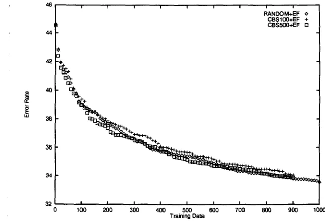
is an error rate of a classifier C s. Thus if there is an increase or no reduction in the error rate after adding an example e to the training set, a clas- sifter goes back to the state before the change.

As Figure 2 shows, the error feedback pro- duced a drastic reduction in the error rate. At 900, the committee-based m e t h o d with the error feedback reduced the error rate by as much as 23%. Figure 3 compares performance of three sampling methods, random sampling, the committee-based sampling with 100 bootstrap replicates

(i.e.,

K = 100) and that with 500

(8)

Figure 2: The committee-based method (with 100 bootstraps) with the error feedback as compared against one without. The error rate decreases rapidly with the growth of the training data (the lower scatterplot). The upper scatterplot represents CBS with the error feedback disabled.

46

44'

42

uJ

38

36

34 0

o o C~+C4.5 o

0 4 2 0 0 CBS.~C4.5+EF +

o o ~ ° °°°oo~ o ~ : o ~ ~ o ooo o ~ % o o o

o ~oo o o o ~ o

~ ° o

\

+

\

++~+%+++++++++++*+-H.++++

+++'H'~'+~'++'~'+÷++++'H

~'H'+++++..H.+++.H..H.~.+

...

I I I I I I I I "J'H'4"l:+,~

100 200 300 400 500 600 700 800 900

Training Data

Figure 3: Comparing performance of three approaches, random sampling (RANDOM-EF), boot- strapped CBS with 100 replicates (CBS100-EF), and bootstrapped CBS with 500 replicates (CBS500-EF),: all with the error feedback on.

42

4 0

3 !

36

34

32

i ,'

RANDOM+EF o

CBS100+EF + CBS500+EF E]

[~÷

| I I I I I I I I

100 200 300 400 500 600 700 800 900

Training Data

1000

amount of training data without hurting perfor- mance.

5 C o n c l u s i o n s

We presented a new approach for identifying discourse relations, built upon the committee-

[image:8.612.141.454.116.336.2] [image:8.612.134.455.396.615.2]

(9)

Figure 4: Differences in performance of RANDOM-EF (random sampling with the error feedback) and CBS500-EF (CBS with the error feedback, with 500 bootstrap replicates).

46

44

42

4O

38

36

34

32

i i i i i i !

random sampling+EF o

C B S + B P S O O + E F +

+o

I I I I I I I I I

100 2 0 0 3 0 0 4 0 0 5(X3 6 0 0 7 0 0 8 0 0 9 0 0

Training Data

1000

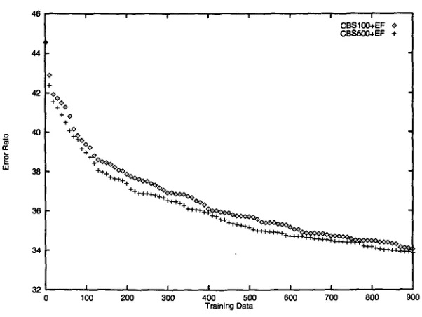
Figure 5: Differences in performance of CBS500-EF and CBS100-EF.

44

4O

38

36

34

! i

C B S l O O + E F ¢.

CBSSOO+EF +

+ o ₊

• ~ ~ + + ~ . : v . , , , ~

3 2 I , I I I I I | I -

0 1 O0 2 0 0 3 0 0 4 0 0 5 0 0 600 700 800 900

Training Data

ing a statistical technique called

bootstrapping.

The use of the method for learning discourse relations resulted in a drastic reduction in the amount of data required and also an increased accuracy. Further, we found that the number of bootstraps has substantial effects on performance; CBS with 500 bootstraps performed better than that with 100 bootstraps

R e f e r e n c e s

Paul R. Cohen. 1995.

Empirical Methods in Ar-

tificial Intelligence.

The MIT Press.

Ido Dagan and Sean Engelson. 1995. Committee-based sampling for training probabilistic classifiers. In

Proceedings off In-

ternational Conference on Machine Learning,

pages 150-157, July.

[image:9.612.165.467.107.328.2] [image:9.612.164.465.360.586.2]

(10)

!

comparison of three methods for constructing ensembles of decision trees: Bagging, boost- ing, and randomization,

submitted to Ma-

chine Learning.

Sean P. Engelson and Ido Dagan. 1996. Mini- mizing manual annotation cost in supervised training from ,corpora. In

Proceedings off the

3~th Annual Meeting of the Association for

Computational Linguistics,

pages 319-326. ACL, June. University of California,Santa

C r u z .

Takashi Ichikawa. 1990.

Bunshddron-gaisetsu.

KySiku-Shuppan, Tokyo.

Klaus Krippendorff. 1980.

Content Analysis:

An Introductiqn to Its Methodology,

volume 5 of

The Sage

COMMTEXT

series.

The Sage Publications, Inc.

W. C. Mann and S. A. Thompson. 1987. Rhetorical Structure Theory. In L. Polyani, editor,

The Structure of Discourse.

Ablex Publishing Co:rp., Norwood, NJ.

Daniel Marcu. 1997. The Rhetorical Pars- ing of Natural Language Texts. In

Proceed-

ings of the 35th Annual Meetings of the As-

sociation for ,Computational Linguistics and

the 8th European Chapter of the Association

for Computational Linguistics,

pages 96-102, Madrid, Spain, July.

Nihon-Keizai-Shimbun- Sha. 1 9 9 5 . Nihon Keizai Shimbun 95 hen CD-ROM ban. CD-ROM. Nihon Keizai Shimbun, Inc., Tokyo.

J. Ross Quinlani 1993.

C~.5: Programs for Ma-

chine Learning.

Morgan Kanfmann.

Gerald Salton and Michael J. McGill. 1983.

Introduction t o Modern Information Re-

treival.

McGraw-Hill Computer Science Se- ries. McGraw~Hill Publishing Co.

Ken Samuel, Sandra Carberry, and K. Vijay- Shanker. 1998. Diaglogue act tagging with transformation-based learning. In

Proceed-

ings of the 36th Annual Meeting off the Asso-

ciation of Computational Linguistics and the

17th International Conference on Computa-

tional Linguistics,

pages 1150-1156, August 10-14. Montreal, Canada.

Sidney Siegel and N. John CasteUan. 1988.