Abstract— A novel method of on-line flame detection in video is proposed. It aims to early detect the current state of the combustion system and prevent the system from further degradation and occurrence of failure. The proposed method consists of hidden Markov model (HMM) and multiway principal component analysis (MPCA). MPCA is used to extract the cross-correlation among spatial relationships in the low dimensional space while HMM constructs the temporal behavior of the sequence of the spatial features. The probability distribution of the normal status can be trained by the images collected from the normal operation processes. The proposed method can generate simple probability monitoring charts to track the progress of the current transition state sequence and monitor the occurrence of the observable upsets. To demonstrate the performance of the proposed method, data from the monitoring practice in the real combustion systems are conducted.
Index Terms— Combustion Systems; Hidden Markov Model; Multiway Principal Component Analysis; Statistical Process Control
I. INTRODUCTION
The industrial furnaces, such as fossil fuel-fired furnaces, are widely used to produce electrical power by combusting different fuels [1]. Many combustion problems, including poor flame stability, low combustion efficiency and high pollutant emissions, should be considered. Therefore, the monitoring of combustion processes have become highly desirable to monitor, estimate and even reduce the levels of pollutant emissions [2,3].
One traditional way to monitor the combustion process is flame watch by experienced workers. Nevertheless, the drawbacks are that it is hard to quantify the combustion performance only by human experience and the working environment is usually too poor [4]. Temperature is a general measurement index to monitoring the combustion process. The conventional temperature monitoring devices, such as thermocouples and pyrometers, are single-point measurement and cannot provide the temperature distribution of the flame. With the current development of optical sensing and digital image processing techniques, on-line continuous monitoring of the flame is becoming possible by a spatial and
This work was sponsored in part by National Science Council, R.O.C. and in part by the project Toward Sustainable Green Technology in the Chung Yuan Christian University, Taiwan, under grant CYCU-98-CR-CE
J. Chen is with Department of Chemical Engineering, Chung-Yuan Christian University, Chung-Li, Taiwan 320, Republic of China (corresponding author to provide fax: 886-3-265-4199; e-mail: jason@ wavenet.cycu.edu.tw).
T.-Y. Hsu is with Department of Chemical Engineering, Chung-Yuan Christian University, Chung-Li, Taiwan 320, Republic of China.
cost-effective way [3].
Some researchers developed statistical sensitivity methods to monitor the combustion process. Yan et al. (2002) extracted the geometrical and luminous features of the pulverized coal flames to quantify the combustion process and did sensitivity analysis [1]. They demonstrated that some image features could help detect the change of combustion processes. However, most research focused only on the point estimation without considering the region of operating distribution. Whereas an incipient fault occurs in the operation combustor, fault information is often weak; it is difficult to extract weak fault information using direct analysis of the image data because in practice, the flame flicker frequency is not constant and it varies with time. Therefore, it is necessary to create a new process control method to monitor the combustion process.
Hidden Markov models (HMM) are recognized as being appropriate for time sequence data. In a HMM model, each observation is the data sequence depending on the previous elements in the sequence. An HMM is capable of characterizing a doubly embedded stochastic process with an underlying stochastic process that can be observed through another set of stochastic processes because the state of the system is not observable directly [5]. With the inspiration of the HMM framework, a statistical model of spatiotemporal dynamic process variables for the sequence images is developed using HMM and MPCA in this paper. The dynamic data array is constructed by incorporating both static and dynamic image characteristics using the prior and the current images. The strongest relations of the scores are extracted by MPCA. With the extracted scores, the HMM model can be integrated into the existing MPCA method to enhance the capability of statistical process monitoring. Thus, the control chart for a two-dimensional image is developed in this research. The chart is not only an analysis the two-dimensional spatiotemporal measurements but also capture the statistical characteristics of the practical data.
II. MPCA-HMMBASED MODELING FOR DYNAMIC IMAGES Flame images exhibit spatially homogeneous repetitions and temporally dynamic patterns. The repetition is the pattern of the burning flame that changes regularly its amplitude, form and color. The sequences of images show a regular pattern repetition and dynamic behavior because this repetition can be found in time as well as in space. This means that each flame image is seen as a point in a given subspace, following a trajectory as time evolves. The modeling dynamic images can locate an appropriate subspace to represent the trajectory and identify the stochastic
Image Based Monitoring for
Combustion Systems
trajectory with a method of dynamic stochastic theory. In this research, an integrated image-based model that makes use of two statistic techniques, MPCA and HMM, to describe the spatial and temporal behavior is proposed for monitoring the operation combustors. MPCA is used to extract the spatial features of the trajectory in a smaller space while HMM is used to train temporal behavior using a dynamic probability model.
A. Spatial Feature Extraction: MPCA
The data set of a sequence of τ images can be arranged as a two-dimensional array as shown in Fig. 1. Assume each color image of the size is N1×N2 and the original color encoding is RGB. It can be reshaped into a sequence of column vectors of the length M =N1×N2×3 . With a sequence of τ color images, the column vectors ( M
k∈R
x ,
1, ,
k= L τ ) are ordered from top to the bottom in a two-dimensional array 1
T M
R τ
τ ×
⎡ ⎤
=⎣ ⎦ ∈
X x L x , where
lower indices indicate that the matrix collects frames from 1
to τ . The temporal mean of each pixel is computed and subtracted from X, and a new matrix Y is obtained. To get the information on the variability among the images, MPCA is performed,
1 2
3
M= N N
2 N 1 N
1
T x
2
T x
time
time
M
Y
1
T x
2
T x
T
τ
x Image τ
T
τ
[image:2.595.57.291.388.587.2]x
Fig. 1. Unfolded structures of the dynamic textures
1
R
T
r r
r=
=
∑
+ = +Y t p E TP E (1)
where R is the number of principal components, E is a residual matrix, and T represents the score matrix
11 12 1 1
1 2
1 2
T
R
T
k k kR
k
T
R
t t t
t t t
tτ tτ tτ
τ
⎡ ⎤ ⎡ ⎤
⎢ ⎥ ⎢ ⎥
⎢ ⎥ ⎢ ⎥
⎢ ⎥ ⎢ ⎥
= =
⎢ ⎥ ⎢ ⎥
⎢ ⎥ ⎢ ⎥
⎢ ⎥ ⎢⎣ ⎥⎦
⎣ ⎦
t
T t
t
L M M
M M
L
(2)
and P=
[
p1 p2 L pR]
is the loading matrix. This meansthat dimension reduction is performed by retaining the first R single value of the decomposition. Thus each frame is written as
1 1 2 2
ˆ
T T T T T
k = k + k =tk +tk + +tkR R+ k
y y e p p L p e
(3)
This means that ˆT k
y is a linear combination of the columns of matrix P, which contains the basis of the subspace onto which the image vector yTk is projected. The columns of
matrix P contain the eigenvectors whose linear combination generates one flame image. The score vector T
k
t fixes the weights of the linear combination, so the features of image frames changed in time are extracted. ek represents the
residual error.
B. Temporal Feature Extraction: HMM
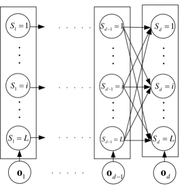
HMM illustrated in Fig. 2 is a double stochastic model, where the non-boxed circles represent a sequence of observations. When HMM is applied to the combustor system, the method for modeling sequential image data is the chain structure that captures interaction between a sequence of inputs,
1 o
1
S =L
1
S =i
1 1
S =
1 d− o
1
d
S− =L
1 d S− =i
1 1 d
S− =
d o
d
S =L
d
S =i
1
d
[image:2.595.343.519.492.674.2]S =
Fig. 2. Graphical model for HMM with the sequential variables
1, 2, ,
T
k = ⎣⎡t k t k tR k vk⎤⎦
o L
(4)
where ok consists of extracted tr k, , r=1, 2,L ,R over the
corresponding residual variation at time point k, which is defined as
T
k k k
v =e e
(5) To capture the interaction in the sequence data, the number of the past τ observation is used to train HMM. First the feature data from the MPCA decomposition,
{
o1 o2 L oτ}
is collected. In Fig. 2, there is a set ofhidden variables, s=
{
S1,L ,Sd}
, and a fixed number of states (L). The probability P( )o can be written as a sum of term P(o s) over all the possible state sequences,all s 1 1 ( ) ( ) ( | ) ( ) ( ) ( ) K
k k k k
k
P P
P P
P S P S S − = = = ⋅ = Π
∑
∑
∑
s so o s
o s s
o
(6)
The transition distribution (P S S( k k−1)) is defined as
1 2
1 1 2
( k k ) j j
P S = j S − = j =a , 1≤ j j1, 2 ≤L
(7) Thus the probability of the transition,
{ }
1 2 j j a
=
A , is an
L L× state transition probability matrix. Note that at the starting point, the initial state distribution, Π =
{ }
πj and1
( )
j P S j
π = = . The observation distribution (P(ok Sk)) is characterized by a mixture of Gaussian density
1
( ) ( , )
H
k k jh jh jh
h
P S j c N
=
= =
∑
o μ Σ
and
1
1, 0, 1, 2, , H
jh jh
h
c c j L
=
= ≥ =
∑
K(8)
where H is the number of mixtures. c is the weight for each mixture component but it should sum up to 1 for each state. Each Gaussian probability density function is an elliptically symmetric density with the mean vector μjh and the
covariance matrix Σjh . The observation probability
parameters are B=
{
cjh,μjh,Σjh}
. For detail in mixture ofGaussian distribution, please refer to [6]. Thus, the HMM model parameters are λ=
[
A B Π]
. The detail of the training algorithm can be found in [7].Given the above optimization for determining the HMM parameters, λ=
[
A B Π]
, it is necessary to return to the assumption that the window size (d) is known. To determine the window size, the HMM problem should be solved in Eq. (6) for several values of d, with the value of d giving the lowest dispersion of a stochastic process,min ( ) min ( k) log( k) k
d H d = − d
∫
p o o do (9)being the best estimate of the window size. The above equation, so called entropy, is a unified probability measure of uncertainty quantification. The main advantage of entropy is that it provides a general description of stochastic system without constraints of certain distribution [8]. This approach, which is essentially a search in one direction, is required because the variable (d) is discrete, so it is not possible to determine the analytical derivation of H d( ) with respect to the window size. The technique is iterative in nature and the search procedure is terminated when minimal relative improvement (
(
H d( )−H d( −1))
H d( −1)) is less than a preset value.11
S= S2=1 22 S= 1 d S= 2 d S= d S=L
1⇒
o
1
d
τ − +
o I⇒
o oτ − +d2 oτ
1
o o2 od
-4 -3 -2 -1 0 1 2 3 4 0 0.05 0.1 0.15 0.2 0.25 0.3 0.35 0.4 0.45 observation (O) b^ ( ) ( h| hopt,)
h t
b=PO S λ
0.95
k k
bd
∈Ω =
∫O O
12
S=
1
S=L S2=L
11
S=
12
S=
1
S=L
21
S=
22
S=
2
S=L
[image:3.595.305.539.291.467.2]1 d S= 2 d S= d S=L
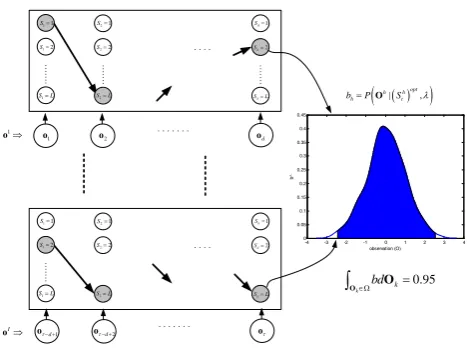
Fig. 3. The optimal state sequence in bold line in the trained model for each data set and the probability of the selected optimal state at the end time point of the moving window forms a distribution.
III. MONITORING CONTROL CHART BASED ON MPCA-HMM
Once the HMM model is trained, the most likely state sequence for an observed sequence could be found. For a given model and an observation sequence
{
1}
k
k d− k− k
=
O o L o o , the most likely underlying state sequence (
( ) {
1 * * * *}
1 1 2 1
d
d
s + = s s L s+ ) can be found
( ) {
}
11
*
1 * * * 1
1 1 2 1 arg max (d , 1 )
d k d
d
s
s s s s P s λ
+
+ +
+
= L = O
the process variables do not perfectly conform to the deterministic model. This variability is resulted from the uncertain variations and disturbances among the lurking variables that affect the system.
For on-line monitoring of the observation images, the control limits should be built for normal operation. As the new image is taken, the image data from the beginning till the current time point (k) are available (Y( )k )
1 1
( ) T T T
k d k k
k = ⎣⎡ − + − ⎤⎦
Y y L y y (11)
The score matrix by projecting the data (Y( )k ) onto the loading matrix (P) can be computed:
( )Tk =Y( )k P (12)
,1 ,2 ,
1,1 1,2 1, 1
,1 ,2 ,
( )
T
k d k d k d R
k d
T
k k k R
k T
k k k R
k
t t t
k
t t t
t t t
− − −
−
− − −
−
⎡ ⎤ ⎡ ⎤
⎢ ⎥ ⎢ ⎥
⎢ ⎥ ⎢ ⎥
= =
⎢ ⎥ ⎢ ⎥
⎢ ⎥ ⎢ ⎥
⎢ ⎥
⎢ ⎥ ⎣ ⎦
⎣ ⎦
t
T t
t
L M M
L L
(13)
The portion of the data (Y( )k ) corresponding to the M−R smallest singular values forms the residual variation
1 1 1
( )
T
k d k d k d
T
k k k
T
k k k
v
k v
v
− − −
− − −
⎡ ⎤
⎡ ⎤
⎢ ⎥
⎢ ⎥
⎢ ⎥
⎢ ⎥
= =⎢ ⎥
⎢ ⎥
⎢ ⎥
⎢ ⎥
⎢ ⎥
⎣ ⎦ ⎣ ⎦
e e
v
e e e e
M M (14)
(
)
1
( )
T k d
T T
k T k
k
−
−
⎡ ⎤
⎢ ⎥
⎢ ⎥ = −
⎢ ⎥
⎢ ⎥
⎢ ⎥
⎣ ⎦
e
I PP Y e
e
M
(15)
Then concatenate the score vector T n
t and the variation vn,
, , 1,
n= −k dL k− k sequentially to make a sequence pool
{
1}
k
k d− k− k
=
O o L o o . With the developed probability distribution that reflects the normal operation, the control limit for the selected state at each time point is required to detect any departure of the process from its standard behavior
( )
( )*
*
( | , ) th ( | , ) 0.95
k k k k k
P s λ>P P s λ d ≤
∫
o o o(16)
This integral is approximated by bootstrapping the original sequential data set to generate enough data and obtain truly quality-related variables from the sequential process data. For more information on the bootstrapping, please refer to work by [10]. The data corresponding to 95% of the confidence limit is taken to get a likelihood threshold ( th
P ).
[image:4.595.305.542.50.205.2]Tim e
Fig. 4. The experimental combustion system.
IV. EXAMPLES
A schematic diagram of the experimental furnace with a flame-monitoring system is shown in Fig. 4. The burner of the experimental furnace uses industrial heavy oil as fuels. The air source of combustion comes directly from a direct-driven air compressor. A digital color camera is installed to capture the images of flames in the furnace. The camera with the specifications of 658×492 pixels and a resolution of 24 bits per pixel is capable of capturing flame images at 73 frames per second. The output signal of the camera is sent to a computer in IEEE-1394a interface and the imaging sample rate is set as one frame per four seconds considering the computer loading.
2 3 4 5 6 7 8 9 10
0 5 10 15 20 25 30 35 40
Window size (d)
R
el
at
iv
e i
m
pr
ov
em
[image:4.595.323.521.449.607.2]ent
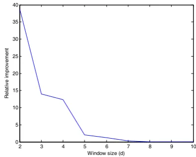
Fig. 5. Entropy of the observation probability
of the variation in the process data set. Then, temporal sequential data are constructed using the extracted features from PCA model. During training HMM, the different window sizes of HMM are applied. Fig. 5 shows the entropy of the observation probability decreases with the increasing number of window sizes. Thus, the selected window size of HMM is 7. The control charts of the models for the normal operation are shown in Fig. 6, where the control limit of log (Pok| )λ is obtained from the proposed MPCA-HMM. The control limits representing 95% and 99% confidence limits are also shown in Fig. 6.
(a)
0 100 200 300 400 500 600 0
200 400 600 800 1000 1200 1400 1600 1800 2000
Time
-log P
(b)
50 100 150 200 250 300 350 400 450 500 550 600 0
10 20 30 40 50 60 70 80 90 100
Time
-log P
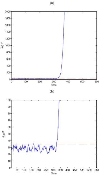
Fig. 6. (a) The testing data monitored by PCA-HMM control charts of the normal operating conditionwith 95% (dash line) and 99% (solid line) confidence limits. The first 300 points are normal and the rest (from 301 to 600), abnormal; (b) zooming in on the data around the control limits.
Two abnormal conditions, which are two different levels of feed air rates linearly decreasing during two different periods of time, are used for testing. For easy visualization and comparisons, time-sequential images in one normal condition and two abnormal ones are shown in Fig. 7. However, differences between the normal (Fig. 7(a)) and the minor abnormal (Fig. 7(b)) operating behaviors can not be distinguished from the image data directly. The spatiotemporal correlations in the image are not apparent because flame flicker frequency which is not constant incurs the variations in flame pixels. To save space limitation, only the minor fault condition is used for testing. The set of 600
observed images, including the first 300 images in the normal condition and the rest 300 in the abnormal one, is used for detection. For the abnormal condition, the monitoring outcomes of the proposed model are shown in Fig. 6. The initial time of the fault is induced at the 301th point. As shown in Fig. 6, even though the abnormal process with small disturbance exists, the fault can still be detected after MPCA-HMM is applied to characterizing the temporal dynamics between images.
(
| opt)
k k
P o S has been increased remarkably and it has fallen outside of the 95% confidence limit after the 320th time point. The small detection lag is due to the transport delay of the air flow.
If the complete training data structure is directly applied to HMM without variable reduction, the number of observed variables are more than 971208 at each time point. The HMM model with 3 hidden states would result in 5827257 parameters, which are a prohibitively large number. It is impossible to train the model. The problem is usually encountered when we have a moderately large number of observed variables. It can be alleviated by the proposed method. In this study, the number of parameters in MPCA-HMM is 51, which is significantly less than that in HMM only. The smaller the number of parameters is fitted, the faster the model training would be converged and the less risk of overfitting the training data would have. Thus, it explains why HMM is used to construct the temporal behavior of the variables after MPCA in the proposed method.
(a)
(b)
[image:5.595.67.270.208.567.2](c)
Fig. 7. Time-sequential images where the interval between the images is three minutes: (a) normal; (b) abnormal with the minor fault condition; (c) abnormal with the major fault condition
V. CONCLUSION
[image:5.595.306.561.427.589.2]fuel consumption. In this paper, HMM based monitoring is proposed. However, the use of HMM in on-line image analysis has up to now been limited to the area of the text and speech recognition. Since the sequences of images from combustors can be regarded as simply two-dimensional signals with the independent variables repeated in the time frame. In this research, the conventional multivariate MPCA are extended by incorporating the HMM structure to solving the detection problem for the two-dimensional repetition observation. In order to quantitatively discriminate the operation distribution, MPCA-HMM is applied at the modeling probability distribution stage. The spatiotemporal patterns can be trained. The corresponding control limits that evaluate the current process can be estimated. Even though the sequence image has a two-dimensional spatial relationship and a temporal behavior, the comparisons of quantitative and qualitative results of the proposed method are made through a real experimental problem for investigating the feasibility of the proposed MPCA-HMM method. The proposed method may be incorporated with different surveillance systems for image monitoring and early detection.
REFERENCES
[1] Y. Yan, G. Lu, and M. Colechin, “Monitoring and characterisation of pulverized coal flames using digital imaging techniques,” Fuel, 81, pp.647-656. 2002.
[2] J.M. Beer. “Combustion technology developments in power generation in response to environmental challenges,” Prog. Energy Combust Sci., 26, pp. 301-327, 2000.
[3] L.Gang, Y. Yong and C. Mike, “A digital imaging based multifunctional flame monitoring system,” IEEE Trans Instrum Meas., 53, pp.1152-1158. 2004.
[4] H. Zhang, Z. Zou, J. Li and X. J. Chen, “Flame image recognition of alumina rotary kiln by artificial neural network and support vector machine methods,” Cent South Univ Techno1., 15, pp.39-43, 2008. [5] L.R. Rabiner, “A tutorial on hidden Markov models and selected
applications in speech recognition,” Proc. IEEE, 76, pp.257-286, 1989 [6] T. Mitchell, Machine Learning, McGrew Hill, New York, 1997. [7] J.M. Lee, S.J. Kim, Y. Hwang and C.S. Song, “Diagnosis of
mechanical fault signal using continuous hidden Markov model,”J Sound Vibrat., 276, pp.1065-1080, 2004.
[8] A. Papoulis, Probability, random variables and stochastic processes, 3rd ed., New York: McGraw-Hill, 1991.
[9] M.D. Moore, “Most Likely state sequence speech reconstruction using a generalized Hidden semi-Markov model with two distinct regeneration times applied to English,” Ph.D dissertation, Rensselear Polytechnic Institute, 2004.