Abstract In CNC milling process, proper setting of cutting



Abstract—In CNC milling process, proper setting of cutting parameter is important to obtain better surface roughness. Unfortunately, conventional try and error method is time consuming as well as high cost. The purpose for this research is to develop mathematical model using multiple regression and artificial neural network model for artificial intelligent method. Spindle speed, feed rate, and depth of cut have been chosen as predictors in order to predict surface roughness. 27 samples were run by using FANUC CNC Milling α-T14E. The experiment is executed by using full-factorial design. Analysis of variances shows that the most significant parameter is feed rate followed by spindle speed and lastly depth of cut. After the predicted surface roughness has been obtained by using both methods, average percentage error is calculated. The mathematical model developed by using multiple regression method shows the accuracy of 86.7% which is reliable to be used in surface roughness prediction. On the other hand, artificial neural network technique shows the accuracy of 93.58% which is feasible and applicable in prediction of surface roughness. The result from this research is useful to be implemented in industry to reduce time and cost in surface roughness prediction.

Keywords—CNC milling, surface roughness, multiple regression, artificial neural network

I. INTRODUCTION

HE challenge of modern machining industries is mainly focused on the achievement of high quality, in term of work piece dimensional accuracy, surface finish, high production rate, less wear on the cutting tools, economy of machining in terms of cost saving and increase of the performance of the product with reduced environmental impact. End milling is a very commonly used machining process in industry. The ability to control the process for better quality of the final product is paramount importance.

The mechanism behind the formation of surface roughness in CNC milling process is very dynamic, complicated, and process dependent. Several factors will influence the final surface roughness in a CNC milling operations such as controllable factors (spindle speed, feed rate and depth of cut) and uncontrollable factors (tool geometry and material properties of both tool and workpiece). Some of the machine operator using ‘trial and error’ method to set-up milling machine cutting conditions (Julie Z.Zhang et al., 2006). This

M.F.F. Ab. Rashid is with the Faculty of Mechanical Engineering, Universiti Malaysia Pahang, Pekan, Malaysia (phone: +6094242256; e-mail: [email protected])

M.R. Abdul Lani was previously with Faculty of Mechanical Engineering, University Malaysia Pahang, Pekan, Malaysia. (email: [email protected])

method is not effective and efficient and the achievement of a desirable value is a repetitive and empirical process that can be very time consuming.

Thus, a mathematical model using statistical method provides a better solution. Multiple regression analysis is suitable to find the best combination of independent variables which is spindle speed, feed rate, and the depth of cut in order to achieve desired surface roughness. Unfortunately, multiple regression model is obtained from a statistical analysis which is have to collect large sample of data. Realizing that matter, Artificial Neural Network (ANN) is state of the art artificial intelligent method that has possibility to enhance the prediction of surface roughness.

This paper will present the application of ANN to predict surface roughness for CNC milling process. The accuracy of ANN to predict surface roughness will be compared with mathematical model that built using multiple regression analysis.

II. LITERATURE REVIEW

Previously, Oktem et al. (2005) proposed the genetic programming approach to predict surface roughness based on cutting parameters (spindle speed, feed rate and depth of cute) and on vibrations between cutting tool and workpiece. From this research, they conclude that the models that involve three cutting parameters and also vibrating, give the most accurate predictions of surface roughness by using genetic programming.

Later on 2007, Chang et al. were established a method to predict surface roughness in-process. In their research, roughness of machined surface was assumed to be generated by the relative motion between tool and workpiece and the geometric factors of a tool. The relative motion caused by the machining process could be measured in process using a cylindrical capacitive displacement sensor (CCDS). The CCDS was installed at the quill of a spindle and the sensing was not disturbed by the cutting. A simple linear regression model was developed to predict surface roughness using the measured signals of relative motion. Surface roughness was predicted from the displacement signal of spindle motion. The linear regression model was proposed and its effectiveness was verified from cutting tests.

Tasdemir et al. (2008) applied ANN to predict surface roughness a turning process. This method was found to be quite effective and utilizes fewer training and testing data.

Surface Roughness Prediction for CNC Milling

Process using Artificial Neural Network

M.F.F. Ab. Rashid and M.R. Abdul Lani

Hazim et.al (2009) developed a surface roughness model in end milling by using Swarm Intelligence. From the studies, data was collected from CNC cutting experiments using Design of Experiments approach. The inputs to the model consist of Feed, Speed and Depth of cut while the output from the model is surface roughness. The model is validated through a comparison of the experimental values with their predicted counterparts.

III. METHODOLOGY

A. Multiple Regression Analysis

After the surface roughness is obtained for all experiments, a table needs to be filled in order to obtain several values for the analysis. In order to obtain regression coefficient estimates β0, β1, β2, and β3, it is necessary to solve the given simultaneous system of linear equations.

i Y i X i X i X

n₀  ₁ ₁  ₂  ₂  ₃ ₃  (1) i Y i X i X i X i X i X i X i

X_{1 1 1}2 _{2 1 2 3 1 3 1}

0       

 (2)

i Y i X i X i X i X i X i X i

X_{2 1 1 2 2 2}2 _{3 2 3 2}

0       

 (3)

i Y i X i X i X i X i X i X i

X_{3 1 1 3 2 2 3 3 3}2 ₃

0       

 (4)

The simultaneous system of linear equations above can be simplified into matrix form. The values of regression coefficients estimated can be obtained easier then.

After the simultaneous system of linear equations above is solved the regression coefficient estimates will be substitute to the following regression model for surface roughness.

i X i X i X i

Y ₀_{1 1} _{2 2} _{3 3} (5) Where;

Yi= Surface Roughness (µm)

X1i= Spindle Speed (rpm)

X2i = Feed Rate (mm/min)

X3i = Depth of Cut (mm)

When the mathematical model is obtained, the value of predicted surface roughness for each experiments can be calculated.

B. Artificial Neural Network (ANN)

Artificial Neural Network is an adaptable system that can learn relationships through repeated presentation of data and is capable of generalizing to new, previously unseen data. Some

network should learn from the data.

For this study, the network is given a set of inputs and corresponding desired outputs, and the network tries to learn the input-output relationship by adapting its free parameters.

The activation function f(x) used here is the sigmoid function which is given by:

) exp( 1 1 ) ( x x f  

 (6) Between the input and hidden layer:



 

 m

i i j

u ji x

1



 j = 1 to n (7) and between hidden layer and output layer:



 

 m

j kjuj k x

1  k = 1to i (8) Where;

m = number of input nodes

n = number of hidden nodes

i = number of output nodes

u = input node values

v = hidden node values

ω = synaptic weight

θ = threshold

In back-propagation neural network, the learning algorithm has two phases. First, a training input pattern is presented to the network input layer. The network then propagates the input pattern from layer to layer until the output pattern is generated by the output layer. If this pattern is different from the desired output, an error is calculated and then propagated backwards through the network from the output layer to the input layer. The weights are modified as the error is propagated.

As with any other neural network, a back-propagation one is determined by the connections between the neuron (the network’s architecture), the activation function used by the neurons, and the learning algorithm (or the learning law) that specifies the procedures for adjusting weights.

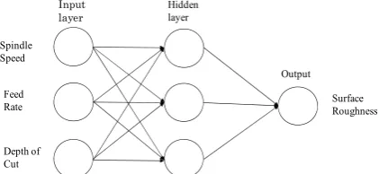
Typically, a back-propagation network is multilayer network that has three or four layers. The layers are fully connected, that is, every neuron in each layer is connected to every other neuron in the adjacent forward layer. Figure 3.2 shows the neural network computational model. The neural network computational model coding is built using MATLAB 2008 software. Output Spindle Speed Feed Rate Depth of Cut Input

layer Hidden layer

C. Experimental Design

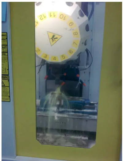
To achieve the project objectives, multiple regression analysis is used for statistical method and Artificial Neural Network is used as artificial intelligent method. The experiment is performs by using a FANUC CNC Milling α -Τ14ιE. The workpiece tested is 6061 Aluminum 400mmx100mmx50mm. The end-milling and four flute high speed steel is chooses as the machining operation and cutting tool. The diameter of the tool is D=10mm. Three levels for each variable are used. For spindle speed 1000, 1250 and 1500 rpm, for feed rate 152, 380 and 588 mm/min, and for depth of cut 0.25, 0.76 and 1.27 mm.

Figure 2: FANUC CNC Milling α-Τ14ιE Workstation For this research, Full Factorial Experiment (FUFE) is applied. Full Factorial Experiment is the experiment where all the possible combinations levels of factors are realized. The table below is the Full Factorial Experiment’s table for this research. The parameters considered are Spindle Speed, Feed Rate, and Depth of Cut. Thus, the numbers of experiment need to be executed are N = 3k _{= 3}3 _{= 27 experiments.}

TABLE 1: THE LEVELS OF EACH PARAMETER Independent

Variables

Levels

Low Medium High Spindle Speed (rpm) 1000 1250 1500 Feed Rate (mm/min) 152 380 588

Depth of Cut (mm) 0.25 0.76 1.27

IV. RESULTS

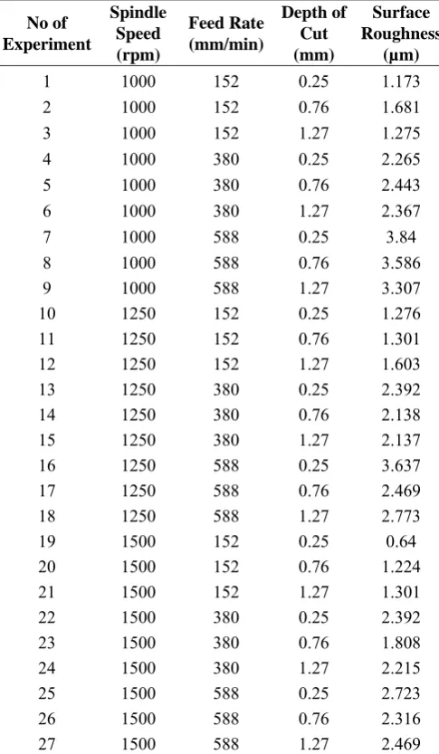
Surface roughness for each experiment is measured using portable surface finish tester, Perthometer S2. All the data taken from the experiment are shown in Table 2.

A. Multiple Regression Analysis Model

Since the surface roughness from the experiment has been established, the analysis for multiple regression using Equation xx above is done to obtain regression coefficient β0, β1, β2, and β3. The sum values calculated for X1,

ΣX1i = 33750 ΣX2i = 10080 ΣX3i = 20.52 ΣYi = 58.751 ΣX1i2 _{= 43312500}

ΣX2i2 _{= 4619232}

ΣX3i2 _{= 20.277}

ΣX1iX2i = 12600000 ΣX1iX3i = 25650 ΣX2iX3i = 7660.8 ΣX1iYi = 72226.5 ΣX2iYi = 25350.268 ΣX3iYi = 44.19635

Substituting all the sums values into the simultaneous equation of linear system (Equation 1-4)

751 . 58 ) 52 . 20 ( ) 10080 ( ) 33750 ( ) 27

( ₀₁ ₂ ₃ 

5 . 72226 ) 25650 ( 12600000) ( 43312500) ( ) 33750

( _{1 2 3}

0    

 268 . 25350 ) 8 . 7660 ( ) 4619232 ( ) 12600000 ( ) 10080

( _{1 2 3}

0    

 19635 . 44 ) 277 . 20 ( ) 8 . 7660 ( ) 25650 ( ) 52 . 20

( _{1 2 3}

0    



Transform above equations into matrix form;

                                         19635 . 44 268 . 25350 5 . 72226 751 . 58 277 . 20 8 . 7660 25650 52 . 20 8 . 7660 4619232 12600000 10080 25650 12600000 43312500 33750 52 . 20 10080 33750 27 3 2 1 0    

After completing the solution for the matrix form, the regression coefficients estimated are;

β0 = 2.1066

β1 = -0.0011

β2 = 0.0040

TABLE 2: SURFACE ROUGHNESS OBTAINED FROM THE EXPERIMENTS

No of Experiment

Spindle Speed (rpm)

Feed Rate (mm/min)

Depth of Cut (mm)

Surface Roughness

(µm)

1 1000 152 0.25 1.173

2 1000 152 0.76 1.681

3 1000 152 1.27 1.275

4 1000 380 0.25 2.265

5 1000 380 0.76 2.443

6 1000 380 1.27 2.367

7 1000 588 0.25 3.84

8 1000 588 0.76 3.586

9 1000 588 1.27 3.307

10 1250 152 0.25 1.276

11 1250 152 0.76 1.301

12 1250 152 1.27 1.603

13 1250 380 0.25 2.392

14 1250 380 0.76 2.138

15 1250 380 1.27 2.137

16 1250 588 0.25 3.637

17 1250 588 0.76 2.469

18 1250 588 1.27 2.773

19 1500 152 0.25 0.64

20 1500 152 0.76 1.224

21 1500 152 1.27 1.301

22 1500 380 0.25 2.392

23 1500 380 0.76 1.808

24 1500 380 1.27 2.215

25 1500 588 0.25 2.723

26 1500 588 0.76 2.316

27 1500 588 1.27 2.469

Then, the regression coefficient can be substituted into the general equation for multiple regression which shown as equation 3.5 in previous chapter. The mathematical model obtains to predict surface roughness is;

Ŷ= 2.1066 – 0.0011X1 + 0.0040X2 – 0.00971X3 (9) Where;

Ŷ= Surface Roughness (µm)

X1 = Spindle Speed (rpm)

X2 = Feed Rate (mm/min)

X3 = Depth of Cut (mm)

B. ANN Model

Besides using multiple regression in surface roughness prediction, artificial neural network a branch of artificial intelligent has been implemented as an alternative approach. The predicted surface roughness has been perform using artificial neural network code in MATLAB® 2008. Table 4.6 shows the predicted surface roughness using this method. The input data for three independent variables spindle speed, feed rate, and depth of cut while actual surface roughness acted as target. The network propagates the input pattern from layer to layer until the output is generated. Then the result output will be compared with the target which is actual surface roughness in this study. The error is calculated and propagated back through network. Then, the weight will be changed and the same process repeated until the smallest error is achieved.

The plot of predicted surface roughness (output) against the actual surface roughness (target) in Figure 3 below shown that both are correlated. This is because the predicted surface roughness is approaching towards the actual surface roughness with the coefficient of determination, R is 0.98508.

Figure 3: Predicted surface roughness against the actual surface roughness

Table 3 shows comparison between actual and predicted surface roughness using multiple regression analysis (MRA) and artificial neural network (ANN). To measure the accuracy for both prediction models, average error for both models is calculated as follows.

% 100

  



i i i i

Ra Ra Ra

Where; i



Ra = Experimental surface roughness



i

Ra = Predicted surface roughness

TABLE 3: COMPARISON BETWEEN ACTUAL AND PREDICTED SURFACE ROUGHNESS

No of Experiment

Actual Surface Roughness

(µm)

Predicted Surface Roughness (µm)

MRA ANN

1 1.173 1.590325 1.1309

2 1.681 1.540804 1.518

3 1.275 1.491283 1.5166

4 2.265 2.502325 2.3069

5 2.443 2.452804 2.6525

6 2.367 2.403283 2.3639

7 3.84 3.334325 3.8318

8 3.586 3.284804 3.645

9 3.307 3.235283 3.2751

10 1.276 1.315325 1.2533

11 1.301 1.265804 1.3074

12 1.603 1.216283 1.6102

13 2.392 2.227325 2.4619

14 2.138 2.177804 2.3222

15 2.137 2.128283 2.0358

16 3.637 3.059325 3.5351

17 2.469 3.009804 2.5429

18 2.773 2.960283 2.6877

19 0.64 1.040325 0.824

20 1.224 0.990804 0.9998

21 1.301 0.941283 1.1844

22 2.392 1.952325 2.3616

23 1.808 1.902804 1.9984

24 2.215 1.853283 1.996

25 2.723 2.784325 2.5754

26 2.316 2.734804 2.6396

27 2.469 2.685283 2.5402

From the average percentage error calculated, the effectiveness of each method can be determined and can be compared.

m m i i

 1

 (11)

Where;

 = Average percentage error

m = number of experiments

For this problem, average percentage error for MRA model is 13.3%, while for ANN model, the average percentage error is 6.42%.

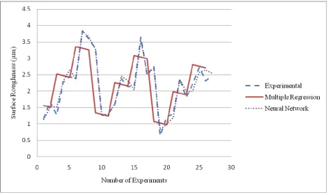
Figure 4 shows the plot of predicted surface roughness using multiple regression analysis and neural network, and actual surface roughness. It shows that the value predicted using neural network predict closely with the actual surface roughness obtained from experiment. Nevertheless, the prediction using multiple regression is also reliable and can be accepted as a successive method.

V. CONCLUSION

The main purpose of this research is to provide an effective and accurate way to predict surface roughness in CNC end milling.

Multiple regression analysis had been applied to develop a mathematical model for surface roughness prediction method. The result of average percentage error is 13.3%, showing that the prediction accuracy is about 86.7%. That means the model developed is reliable to predict surface roughness with accepting accuracy range based on previous research.

Figure 4: Plot of predicted using multiple regression and neural network and actual experimental surface roughness

REFERENCES

[1] B. Smith, “An approach to graphs of linear forms (Unpublished work style),” unpublished.

[2] Chang H.K., Kim J.H., Kim I.H., Jang D.Y. and Han D.C., 2007, “In-process surface roughness prediction using displacement signals from spindle motion”, International Journal of Machine Tools and Manufacture Volume 47, Issue 6,

[3] G. O. Young, “Synthetic structure of industrial plastics (Book style with paper title and editor),” in Plastics, 2nd ed. vol. 3, J. Peters, Ed. New York: McGraw-Hill, 1964, pp. 15–64.

[4] H. El-Mounyari, Z. Dugla, H. Deng. Prediction of surface roughness in end milling using swarm intelligence.

[5] H. Oktem, T. Erzurumlu & F. Erzincanli. 2005. Prediction of minimum surface roughness in end milling mold parts using neural network and Genetic Algorithm. Materials & Design, Volume 27, Issue 9, 2006, Pages 735-744.

[6] H. Poor, An Introduction to Signal Detection and Estimation. New York: Springer-Verlag, 1985, ch. 4.

[7] Hazim El-Mounayri, Zakir Dugla, and Haiyan Deng, 2003,"Prediction of Surface Roughness in End Milling using Swarm Intelligence, IEEE, Indianapolis, USA.

[8] J.Z. Zhang, J.C. Chen & E.D. Kirby. 2006. Surface Roughness optimization in an end milling operation using the Taguchi design method.

[9] M. Brezocnik, M. Kovacic & M. Ficko. 2004. M.D. Savage & J.C. Chen. 2001. Multiple regression-based multilevel in process surface roughness recognition system in milling operations.

[10] Mansour, A. and Abdalla, H. 2002. Surface Roughness model for end milling: A semifree cutting carbon casehardening steel (EN32) in dry condition. Journal of Materials Processing Technology. 124(1-2): pp 183-191.

[11] Medsker, L.R and Liebouwitz, J. 1994. Design and development of expert system and neural computing. New York: Mcmillan College

[12] Negnevitsky, M. 2004. Artificial Intelligent: A guide to intelligent systems. 2nd _{ed. New York: Addison Wesley Publishing.}

[13] S. Tasdemir, S. Neseli, S. Sarıtas, S. Yaldız. 2008. Prediction of surface roughness using artificial neural network in lathe, ACM International Conference Proceeding Series; Vol. 374, Proceedings of the 9th International Conference on Computer Systems and Technologies and Workshop for PhD Students in Computing.

[14] Shepherd, G.M. and Koch, C. 1990. Introduction to synapstic circuit, the synapstic organization of the brain. New York: Oxford University Press. [15] W. Wang, S.H, Kweon & S.H. Yang. 2005. A study on roughness of the

micro-end milled surface produce by a miniatured machine tool. [16] W.-K. Chen, Linear Networks and Systems (Book style). Belmont, CA: