Abstract— The paper describes a conducted research in order to create the scheduling system for electroplating lines. We are interested in an order driven production organization. This type of production requires scheduling in the real-time. In order to avoid costly scheduling, we prepare a set of production scenarios. We use recognition methods to select the most appropriate scenario. Selected scenarios are parameters to a heuristic scheduling algorithm called cyclogram unfolding. We present the short problem notion and algorithm steps. The real-life production line located at Wrocław, Poland is used to explain the algorithm step by step. We analyze the results for historical runs and generated problems.
Index Terms—dynamic hoist scheduling problem, electroplating, scheduling, real-time systems.
I. INTRODUCTION
In electroplating industry a HSP – the Hoist Scheduling Problem occurs. The problem lies in creating a proper schedule for machines working on a production line. On electroplating lines items are chemically processed. The items are transported from a workstation to a workstation by automated hoists. An electroplating line can produce multiple item types. Each has its own sequence of visiting workstations, processing intervals, etc. The production can be organized cyclically and dynamic (the Dynamic Hoist Scheduling Problem - DHSP) - order driven. In the cyclic production a static schedule, called a cyclogram, is repeated in order to produce items. Such organization has its advantages, like simplicity and predictability, but lack in flexibility. In DHSP, schedule is created during production. Produced items vary both in type and time of introduction to line. We present the scheduling system, which divides the problem to the Local Problem[1] where schedules are created with no real-time constraints and the real-time part. Real-time part reacts on new item orders, verifies the feasibility of schedules and implements schedules to line automatons.
II. DYNAMICHOISTSCHEDULINGPROBLEM Electroplating lines cover processed items with thin
Manuscript received May 9, 2010.
Krzysztof Kujawski. is with the Institute of Informatics, Wrocław University of Technology Wybrzeże Wyspiańskiego 27, 50-370 Wrocław, Poland, tel. +48 501306091; e-mail: krzysztof.kujawski@ pwr.wroc.pl.
Jerzy Świątek. is with the Institute of Informatics, Wrocław University of Technology Wybrzeże Wyspiańskiego 27, 50-370 Wrocław, Poland, tel. +48 501306091; e-mail: jerzy.świątek@ pwr.wroc.pl
material coatings using chemical reactions – usually by galvanization. They are automated production systems, which use hoists as transportation. Production line is made of series of workstations. Workstations are capable of performing different elementary chemical reactions or material processing operations. Input product is subjected to several reactions in specific sequence.
Production line consists of: Baths (tanks) and Hoists. Baths are workstations that perform a certain stage of the chemical or material processing. Groups of uniform workstations are also considered. Some workstations can perform more than one stage in processing. Baths are arranged in line, and they create an axis of hoist movement. Hoists – automatons controlled by schedule. Hoists are capable of transferring products between workstations. Hoists move only in production line axis. Hoists cannot pass each other. A hoist can pick up and put down products to workstation. Hoists cannot pass products between each other. The processing starts when a hoist plunge item to a bath. This happens because of the chemical nature of the processing. When a hoist plunge an item to workstation we refer to it as the operation of putting down of an item. The processing stops, when the hoist picks item out of a bath.
In order to increase flexibility of the production system, some production lines are designed to produce many item types. This is done by composing workstations, which are required to produce the certain type of item. Scheduling item types differ in sequence of visited workstations and times of processing at those workstations. In case of chemical processing, instead of time of processing at a certain workstation, we have quality constrains. It means that an item is immersed in the workstation for at least given minimum time and no longer than given maximum time.
One of the first papers about HSP [2] describes the simple application, where the production line has only one hoist and simple sequence of production - always to next workstation. More recent publications [3][4][5] expanded the problem to multiple hoists, [6][7] an arbitrary production sequence, groups of workstations, multifunctional baths[7]. Mentioned papers describe creating of cyclograms in the cyclically organized production. The latest papers that introduce DHSP also vary in details. Some limit the problem to a single hoist [8] or do not consider workstation groups [9]. However, all papers propose some non-exact methods - heuristics. This is understandable, because [10] proved that HSP is NP-Hard type of decisive problems and calculation effort is too big for the real-time calculations in DHSP.
Intelligent Scenario Selection in Dynamic Hoist
Scheduling Problem: The Real-Life
Electroplating Production Line Case Analysis
Fig. 1 The Electroplating Line Overview
The Fig.1 presents a (rather small) typical production line with two hoists, eight workstations, some items during processing, one picked up by the hoist, and a few waiting in the processing queue.
In the cyclic production, an item must be available in a loading station every given interval of time. You cannot immediately change the item type. Due to the cyclic production, a line gradually is loaded with items and after a few cycles the line is full and produces one item each cycle. If we want to change the produced item type, the line must be unloaded - no item is introduced at the loading station and after the same number of cycles the line is empty, and we can start producing new item type. If we are interested in producing many item types together, we have to accept such a costly line loading unloading phase. We may also switch the production to the order driven.
We are going to present a solution for the dynamic problem, supporting multiple hoists, many types of items, workstation groups, multifunctional baths, and arbitrary processing sequences.
A. Scheduling system
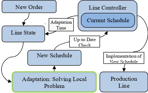
[image:2.595.55.300.633.788.2]The DHSP occurs when the production is performed as described above, but new to-be-produced items availability is not known in advance. We need to maintain a schedule, which includes currently processed items and newly ordered items.
Fig. 2 The Scheduling System
Creation of such schedules is a real-time problem because we cannot halt the production at the time when a new order is specified. If we stopped, the items that are currently processed would break the quality constraints and be destroyed. Therefore, we propose the scheduling system (Fig. 2), which base on the old schedule until it finds a feasible update.
When a new order is stated at moment , the line controller decides about adaptation moment t – time in the
future, from which the schedule changes will be carried on. , 0
t . Line controller provides also information about the line state at the adaptation time according to current schedule. Line state is a parameter to so-called Local Problem [1]. The scheduling algorithm generates a feasible schedule.. Solving the Local Problem lasts of the cyclogram unfolding computation time and produces an updated schedule. Besides other constraints, the updated schedule is the same as the current schedule up to time t. At
this point, the new schedule is checked against its applicability
. In case the updated schedule is infeasible, the scheduling system figures out a new adaptation time and a new Local Problem is solved. When the adaptation is successful, the line controller implements the new schedule to the production line. The line controller converts the schedule to some automaton language e.g. STEP7.B. Notion
The problem of finding the schedule for specified line, queue of items, and line state can be described as optimization problem. The problem parameters are: properties of the line (workstations locations, sizes, workstation counts), hoists count, hoists speed. Other parameters concern produced product types: sequence of workstation for each product type, minimum and maximum times of processing in visited workstations. Additionally, parameters describing the line state in adaptation time: hoist positions, processing stages of products processed, a queue of to be processed items are also considered. A result
New Order Line Controller
Current Schedule Line State
Adaptation: Solving Local Problem
New Schedule
Production Line Adaptation
Time
Up-to-Date Check
schedule can be described by decisive variables of this problem: routes of hoists, assignment of pickup operations to hoists, assignment of put down operations to workstations in groups, times of pickup and put down operations. The optimization criterion is minimizing the time of a last put down operation. Such criterion maximizes the performance of the production line for a given product order. Similarly, to other scheduling problems, DHSP has many constraints. It makes finding any feasible solution very hard. Schedule must fulfill process requirements – processing sequence must be correct, processing times must not be shorter than specified minimum times and longer than specified maximum times. A hoist can carry only one item at the time, a workstation can process only one item at the time. Hoists cannot move outside their physical capabilities, and they cannot collide. We provide only relevant symbols. Extended notion is available in [12].
Parameters are: N – product types count,
1,...,
n N . Z
z1,...,zK
=
o1,...,oKC
1,...,KQ
, the queue of items to be produced. zkN– the type of itemin queue’s k-th place. okN– products, which are already
processed during adaptation. kN– products from new
order, K =KC+KQ. H – the number of hoists present on line,
1,...,
h H . On
w1,...,wi n ,...,wI n
– the sequence ofworkstation group types necessary to manufacture the product of type n. wi n – the processing workstation group
type of an i-th stage of a product type n. i n
1,...I n
where I n
is the number of steps in of product typen
processing sequence. Decisive variables are defined as follows: U h
,
,
1,...,
– routes of hoists, represented as a position of the hoist h in production time .
,
k i z k
t ,tk i z k, – moments of a pick and put of i-th stage of a
k-th product from a queue Z. hk i z k, ,hk i z k, – numbers of
hoists, which perform an i-th pick and put of a k-th product from the queue Z. The optimization criterion is specified as:
,
max k I z k
Q t – the time of last put down of a last
produced item. It is the moment when the line can stop, as none of its resources is used. Optimal solution is found when the criterion reaches minimum. Let
S =
,
0, 1
, , t h H ,
t h
Z P U h t
, ,
,
0, 0
k K i z k I z k
k i z k
k i z k t
,
, ,0, 0 ,
k K i z k I z k
k i z k
k i z k t
,
,
0, 0
k K i z k I z k
k i z k
k i z k h
,
, , 0, 0k K i z k I z k
k i z k
k i z k h
be the schedule for queue Z. Let us mark
S, as the shifting operation. It shifts the schedule S by seconds. The operation changes the schedule variables as defined: tk i z k, tk i z k, ,
, ,
k i z k k i z k
t t ,
, , 0,
, 0 , 0 U h t t U h t
U h t
.
Segmenting operation
Z , divides products from orders to segments of items of the same type, such that:
1,...,KQ
=
s1,1,...,s1,S1
...
sSEG,1,...,sSEG S,SEG
where1,..., i
i SEGS KQ
and, , , 1,..., , 1,...,
i j i m i
s s j m S i SEG . Segmenting divides the new order to sub-sequences of items of the same time. I.e. Z=
1,1,3,1, 2, 2,3,3
means that following segments are created:
1,1 ,
3 ,
1 ,
2, 2 ,
3,3 .It is important to introduce the idea of cyclogram, which is a cornerstone of cyclic production. Cyclogram is a specific type of schedule used in electroplating lines. In [3] authors claim that the cyclic production causes schedule to be periodic. Cyclogram is a schedule that represents one period, a cycle of periodic schedule. Cyclogram contains a constant number of hoist operations. Repeated over and over again, it allows production of any number of items. Cyclograms are built this way, that one item is introduced and completed during one cycle. Main features of cyclogram are a capacity and a cycle time. The cycle time is a length of cyclogram in a time domain. The capacity is a number of cycles needed to be performed in order to load fully a production line and produce a first item. Afterwards, a line produces one new item each cycle. There can be many feasible cyclograms for one item type. Let us assume that there is a number cyclograms for each item type n
1,...,N
referred as1,..., N
V V , vn
1,...,Vn
. T v
n – cycle-time of cyclogramn
v , G v
n – capacity of cyclogram vn. Cyclogram can bedefined similarly as schedules in DHSP – routes, times of operations and assignment of operations to hoists.
n, ,
U v h ,
0,...,T v
n
– routes of hoists,represented as position of the hoist h in production time
for cyclogram vn. t v i n
n,
,t v i n
n,
– moments of pick and put of i-th stage of product n-th in cyclogram vn ,
n,
h v i n ,h v i n
n,
– indexes of hoists which, perform ai-th pick and put of product n-th in cyclogram vn.
Let us mark C x v
, n
as the cyclogram unfold operation, for x items of type n using cyclogram vn. As a result of
, n
C x v we get a schedule based on cyclogram vn, which
produces x items. Cyclogram operations are repeated a number of times until x items leave the line. A schedule
length C x v
, n
=
G vn x T v
n –Tload
vn Tunload
vn . C x v
, n
createsa solution for Z=
z1,...,zx
, where zk n by assignment:
,U h t = U v h t
n, , modT v
n
, t
0,...,C x v
, n
, ,
k i n
t = t v i n
n,
+
k
i n
T v
n ,
( ) 1
1 , ,
0 , ,
a i n n n
a
n n
t v a t v a
i n
t v a t v a
, ,k i n
t =t v i n
n,
+
k
i n
T v
n , where is the
,
k i z k
h =h v i n
n,
, hk i z k, =h v i n
n,
. The cyclogramunfolding is essential for heuristic scheduling method [12]. III. SCENARIO SELECTION
The most difficult part in the scheduling system is solving the Local Problem. This is the true stage where scheduling takes place. We use the Cyclogram Unfolding Method [12] as a basic scheduling algorithm. In current section, we are going to describe an extension to base algorithm.
A. The Cyclogram Unfolding Method The algorithm pseudo-code:
Cyclogram Unfolding
1) Calculate for queue Z
2) for x = 1 to SEG in
s1,1,...,s1,S1
...
sSEG,1,...,sSEG S, SEG
2a) Select arbitrary ,1
x
s
v from
1,..., ,1
x
s
V
2b) Calculate S(x)=
, ,1
x
x s
C S v .
3) Result = CURRENT_SCHEDULE 4) for x = 1 to S
4a) Find smallest t that there
exists collision-less routing
for Result
S x
,
.4b) Result=Result
S x
,
The scheduling system provides necessary parameters: queue Z, adaptation time t current schedule (point 3), and all
the other line specific properties. We prepare cyclogram sets for each type of item before the production starts. Cyclograms can be generated by any cyclic scheduling method available. We use cyclograms generated by the method described in [13] because besides their high performance, they support multiple-hoists, workstation groups, multifunctional tanks, etc. Point 4b) incorporates the routing algorithm. It is the same routing algorithm as described in [13]. In the first iteration, the outermost hoist is forced to drive to the outermost workstation. Next hoists are tracing the previous hoist, staying as close to it as it is possible, while avoiding collisions. In second iteration, we begin from the last hoist and reduce all futile movements. Algorithm is minimizing the hoist route length by using the "central" workstation of the hoist zone to wait when not colliding. Then the post-processing stage eliminates any sequences of hoist movements, which can be replaced by a simple "ride and wait" or "wait and ride" scheme. We use both a constant speed and an acceleration based hoist movement models. An acceleration based model, where a hoist position is calculated with usage of an acceleration ratio, braking ratio and maximum speed is required in real-life applications. In research, like in other papers, we use the constant speed model, where the hoist moves always in maximum speed and can immediately gain such speed and break to stop. Movement models are important in a creation of valid routes for hoists.
Point 2a) includes the decision to make. We used to consider only one cyclogram per item type. We choose a
cyclogram with the shortest cycle-time in presented results. B. The Scenario Selection Method
The Scenario Selection scheduling method assumes that someone experienced in a production process is able to spot regularity in a production state. For example, “it is the best to use particular production method in case we produced many brake pads, and now we are starting to produce ball bearings”. We are trying to gain from domain knowledge of the line. This has its reason. A production line is usually designed once to produce certain types of products. Its design does not change frequently to produce something else. Production orders also may tend to be repeated, as the same customers are ordering.
In DHSP, there are many areas where such assumption would apply. We are interested in point 2a) from the Cyclogram Unfolding Method algorithm. A cyclogram is a scenario that we use to unfold a schedule. We can pick one of many cyclograms present. It is possible to choose the best scenario basing on a situation. This is a typical classification problem. We use the feed-forward, back-propagation artificial neural network in this paper research and calculation of presented results.
For each product type n
1,...,N
, we construct a neuralnetwork n. Network selects a scenario used for unfolding
and shifting operations during scheduling. A number of problem features are calculated to reflect the state of a line and the characteristic of the product order. Features include utilization of workstations, utilization of hoists, a number of products in segment, a length of unfolded segment, a resource collision count. These features are normalized and provided as inputs to the neural network. The algorithm pseudo-code:
Scenario Selection
1) Calculate for queue Z
2) Result = CURRENT_SCHEDULE 3) for x = 1 to SEG in
s1,1,...,s1,S1
...
sSEG,1,...,sSEG S,SEG
3a) Select vsx,1 using sx,1and Result.
If classification is
inconclusive select arbitrary
,1
x
s
v from
1,..., ,1
x
s
V
3b) Calculate S(x)=
, ,1
x
x s
C S v .
3c) Find smallest that there
exists collision-less routing
for Result
S x
,
.3d) Result=Result
S x
,
We use the cyclogram unfolding method for generation of learning examples for the classifier. We generate various line situations and queues and calculate the schedule for each cyclogram from set to check which is best.
IV. ELECTROPLATING LINE CASE ANALYSIS
composed into one column. One group has 3 workstations, and the other groups are in fact, a singular workstation. Two hoists are available. Hoists maximum speed is 0.7 m/s. Hoist collision zone is 2 meters - two hoists centers cannot be closer than 2 meters or the collision occurs.
We will consider two item types that are frequently ordered together. Let us mark the technology process of technical chroming as a "type A" and process of nickeling as a "type B". Table I and Table II define the processes sequence and quality constraints for process, A and B respectfully. All pick up and put down times are 8 seconds.
Table I: The Process A Definition No.
Step
Step name Min.
time
Max. time
Group No.
1 Loading station - - 1
2 Chem. degreasing 300 420 10
3 Dripping 30 90 11
4 Electrochem. degr. 60 180 12
5 Warm rinse 30 90 13
6 Rinse I 20 80 14
7 Cascade rinse I 20 80 15
8 Cascade rinse II 20 80 16
9 Anode etching 150 210 9
10 Chroming 1200 1300 8(3)
11 Salvaging rinse 20 80 7
12 Rinse II 20 80 6
13 Rinse with chrome reduction
20 80 5
14 Rinse III 20 80 4
15 Timed rinse. 20 80 3
16 Blow in bath 30 90 2
17 Unloading station - - 1
[image:5.595.42.296.548.783.2]The step number 10, "Chroming" lasts extensively longer than other steps. For that reason, the chroming bath is multiplied to three workstations. All three workstations can be used in the processing.
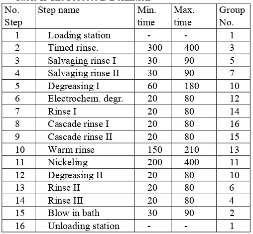
Table II The Process B Definition No.
Step
Step name Min.
time
Max. time
Group No.
1 Loading station - - 1
2 Timed rinse. 300 400 3
3 Salvaging rinse I 30 90 5
4 Salvaging rinse II 30 90 7
5 Degreasing I 60 180 10
6 Electrochem. degr. 20 80 12
7 Rinse I 20 80 14
8 Cascade rinse I 20 80 16
9 Cascade rinse II 20 80 15
10 Warm rinse 150 210 13
11 Nickeling 200 400 11
12 Degreasing II 20 80 10
13 Rinse II 20 80 6
14 Rinse III 20 80 4
15 Blow in bath 30 90 2
16 Unloading station - - 1
To calculate the time required to move a hoist from the workstation, i to j the distance between workstation centers is divided by the maximum hoist speed and rounded up to whole seconds. In order to transport an item from a group hoist need to go to the group center, pick the item up (8 seconds), move to the destination bath and put the item down (8 seconds).
Table III: The Workstation Centers Positions
Group No. 1 2 3 4 5 6
Position (m) 0.3 0.94 1.56 2.18 2.8 3.43 Group No. 7 8(1) 8(2) 8(3) 9 10 Position (m) 4.08 4.85 5.75 6.65 7.46 8.14
Group No. 11 12 13 14 15 16
Position (m) 8.76 9.42 10.08 10.7 11.27 11.79 A. Production
The organization on the line is currently cyclical. The owners want to switch to the dynamic production, because they need to produce many item types together. As a data to research, we will use some historical runs and typical order ratios. For historical runs the schedules are available but without the real-time aspect. We can do it offline as we know the whole order before production is started. Such test is also valuable because it allows benchmarking the performance of created schedules.
Table IV: Queues to Analyze
Queue Items sequence
Queue 1 AABBAABB
Queue 2 7xA;5xB;5xA
Queue 3 20xA;15xB
Queue 4 5xA;5xB;5xA;5xB;5xA
Queue 5 12xB;4xA;6xB;2xA
Queue 6 8xB;8xA
More general production requirements, which we have on the Wrocław line, is that statistically orders are composed like 1:2, so for each item of type Two items of the type B are ordered. We are going to analyze the ratio 2:3 and 1:1.87. For each ratio, the orders are generated. We are going to simulate the real-time production. We generate the queue of 40 items for each proportion (16xA:24xB and 18xA:22xB) with random sequence. We calculate the schedule for three cases: whole order is known at the beginning, the next segment is known in 100 seconds before the shortest available adaptation time, and the next segment is known in the time of the shortest adaptation time. The shortest adaptation time is the time where the last item of current schedule is loaded to line, adaptation time must be greater to keep the correct sequence of item introduction. The result is averaged from 100 generated instances.
B. Algorithm work example
432 sec., capacity 6; and for type B: B1 - length 240 sec., capacity 6; B2 - length 257 sec., capacity 5; B3 - length 532 sec., capacity 3. We have trained two neural networks, each for the different type of item. For the Wrocław line 39 features are extracted from line state, and queue, so neural networks have 39 inputs, 40 neurons in hidden layers and 3 outputs.
Let us analyze the Scenario Selection method for Queue 1. Let us assume that we are starting the production, so the line and schedule are empty. operation gives us four segments {AA}, {BB}, {AA}, {BB}. In the first step1returns A3, S(x) is a production schedule of two items of type A, its length is 2887 seconds. =0 as the current schedule is empty, so there cannot be any collisions. We store the result and proceed to a second iteration. 2 returns B3, We calculate S(x), its length is 1720 seconds. We analyze > 440 seconds and find =893 constructs a feasible schedule for AABB with a length of 2887 seconds. In a third iteration
1
returns A2, We calculate S(x) by cyclogram unfolding, its length is 2967 seconds. We analyze > 1433 seconds and find =2464. We store the result (5431 sec.) and proceed to the last iteration. 2returns again B3, We calculate S(x), its length is 1720 seconds. We analyze > 2896 seconds and find =3424. The schedule for Queue 1 is created and its length is 1:30:31 (5431 sec.). Scheduling takes around 3 seconds. All calculations are performed on Intel Q9300 2.5GHz processor.
V. RESULTS
The tables summarize the results achieved by using the Scenario selection method. In order to show how much time can be gained using calculated schedule, we compare their length to a base solution length. To calculate the base solution length, we sum up all the products minimum times, pick up times, putdown times, and transition times required to produce items from the given queue. The utilization ratio is a length of base solution divided by a length of schedule.
Table V Queues Queue Historical
Schedule Length
Scenario
Selection Improvement Utilization Ratio Queue 1 2:41:36 1:30:31 43.9% 2.44 Queue 2 3:28:48 3:11:32 8.2% 2.81 Queue 3 4:34:51 4:26:05 3.1% 3.97 Queue 4 5:11:12 4:45:21 8.3% 2.59 Queue 5 4:02:48 3:41:36 8.7% 2.47 Queue 6 2:33:24 2:22:14 7.2% 3.12
Table VI Ratio 16:24; The Scenario Selection Test Type Schedule Length Utilization
Ratio
Scheduling Length Entire Order
Known
9:42:56± 1:15:03
2.05±0.20 0:14:20± 0:05:36 100 Seconds
Before
11:09:50±0:18:0 4
1.76±0.03 0:00:27 per segment Adaptation
Time
11:08:29±0:12:1 8
[image:6.595.303.555.62.165.2]1.76±0.03 0:00:27 per segment
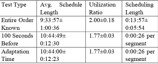
Table VII Ratio 18:22; The Scenario Selection Test Type Avg. Schedule
Length
Utilization Ratio
Scheduling Length Entire Order
Known
9:33:57± 1:00:36
2.00±0.18 0:13:57± 0:05:54 100 Seconds
Before
10:44:49± 0:12:30
1.77±0.03 0:00:26 per segment Adaptation
Time
10:44:00± 0:12:23
[image:6.595.302.555.237.338.2]1.77±0.03 0:00:26 per segment To compare the new algorithm of Scenario Selection to its base the Cyclogram Unfolding, we scheduled the same test cases. Without the selection stage, we use the A1 and the B1.
Table VIII Ratio 16:24; The Cyclogram Unfolding Test Type Schedule Length Utilization
Ratio
Scheduling Length Entire Order
Known
10:47:03± 0:39:12
1.83±0.11 0:20:08± 0:12:37 100 Seconds
Before
13:16:11± 0:18:13
1.48±0.03 0:01:00 per segment Adaptation
Time
13:19:27± 0:18:53
1.47±0.03 0:01:00 per segment Table IX Ratio 18:22; The Cyclogram Unfolding Test Type Avg. Schedule
Length
Utilization Ratio
Scheduling Length Entire Order
Known
10:51:04± 0:37:40
1.76±0.10 0:17:11± 0:11:11 100 Seconds
Before
12:58:18± 0:17:45
1.47±0.03 0:00:59 per segment Adaptation
Time
12:59:13± 0:17:11
1.47±0.03 0:00:59 per segment The utilization ratio higher than 2.0 shows, that statistically the line allows production of at least two products at time. The scheduling length for test "Entire Order Known" is a length of scheduling all the forty items. The scheduling length for other tests shows an average length of updating a schedule with next order (segment in this case).
The scheduling algorithm is efficient enough for the Wrocław line and possibly for similar sized productions. During tests, there were no cases, where the new schedule was out of date and required new adaptation time.
REFERENCES
[1] Lamothe, J., Thierry, C., Delmas, J., A multihoist model for the real time hoist scheduling problem, Proceedings of CESA’96, Lille, France, 9–12 July, 461–466 (1996)
[2] Phillips, L.W., Unger P.S., Mathematical programming solution of a hoist scheduling problem. AIIE Transactions 8 (2), 219–225 (1976) [3] Varnier, C., Bachelu, A., Baptiste, P., 1997, Resolution of the cyclic
multi-hoists scheduling problem with overlapping partitions, INFOR,
35(4), 309–324.
[4] Yan P., Chu C., Che A., Yang N., 2008, Algorithm for optimal cyclic scheduling in a robotic cell with flexible processing times,
IEEE-Proceedings of IEEM'08 Singapore, 153-157
[5] Liu, J., Jiang, Y., Zhou, Z., 2002, Cyclic scheduling of a single hoist in extended electroplating lines: a comprehensive integer programming solution, IIETransactions, 34, 905-914
processing sequences, IEEE Transactions on Robotics and Automation, 19 (3), 480–484
[7] Mak, R.T., Gupta, S.M., Lam, K., 2002, Modeling of material handling hoist operations in a PCB manufacturing facility, Journal of Electronics Manufacturing, 11 (1), 33–50
[8] Hindi, K., Fleszar, K., A constraint propagation heuristic for the single-hoist, multiple-products scheduling problem, Computers & Industrial Engineering 47, 91–101 (2004)
[9] Jegou, D., Kim, D., Baptiste, P., Lee, K., A contract net based intelligent agent system for solving the reactive hoist scheduling problem, Expert Systems with Applications 30, 156–167 (2006) [10] Lei, L., Wang, TJ., A Proof - the Cyclic Hoist Scheduling Problem Is
NP-Hard. Working paper 89-0016, Rutgers University (1989). [11] Paul, H., Bierwirth, C., Kopfer, H.. A heuristic scheduling procedure
for multi-item hoist production lines, International Journal of Production Economics 105, 54–69 (2007)
[12] Kujawski, K., Świątek, J., Using Cyclogram Unfolding in Dynamic Hoist Scheduling Problem, Proceedings of the International Conference on Systems Engineering ICSE’09, UK, Coventry, 282– 287 (2009)