A. Early stopping

Abstract— Intrinsic qualities of the cascade correlation algorithm make it a popular choice for many researchers wishing to utilize neural networks. Problems arise when the outputs required are highly multimodal over the input domain. The mean squared error of the approximation increases significantly as the number of modes increases. By applying ensembling and early stopping, we show that this error can be reduced by a factor of three. We also present a new technique based on subdivision that we call patchworking. When used in combination with early stopping and ensembling the mean improvement in error is over 10 in some cases.

Index Terms—Cascade correlation, early stopping, ensembling, multimodal functions, subdivision method,

I. INTRODUCTION

Neural networks are commonly used for regression modelling, however a perennial problem in the specification is determining the topology of the network. Because hand crafting this structure is very time consuming, growing topology neural networks have gained in popularity. Cascade correlation [1] is a well known member of the constructive types, with hundreds of associated publications each year.

Rather than requiring the designer to answer questions such as:- how many hidden layers, how many neurons in each layer, and which activation functions should be used, cascade correlation automatically makes these choices during its supervised learning process.

The first version of cascade correlation was intended to work best as a classifier but, subsequently, its author made some minor changes that improved its performance in regression roles [2]. The new algorithm was named “Cascade II” but is referred to in this paper as “CasCor”.

The aim of this paper is to study mechanisms that improve the fit of the CasCor neural network - with specific attention to multimodal surfaces. Test functions for global optimisation were being used by the current authors to create training surfaces, and curiosity grew as to why certain

Manuscript received March 10, 2010. This work was supported by an EPSRC Doctoral Training Grant.

Mike J. W. Riley is a Doctoral Research Student in the School of Engineering, Cranfield University, Cranfield, Bedford MK43 0AL, UK. (e-mail: [email protected]).

Chris P. Thompson is the head of the Applied Mathematics and Computing Group and the Professor of Applied Computation at Cranfield University. (e-mail: [email protected])

Karl W. Jenkins is a lecturer in the Applied Mathematics and Computing group of Cranfield University and specializes in computational engineering. (e-mail: [email protected]).

functions caused exceptional mapping problems for CasCor neural networks. Whilst undertaking work to resolve these problems, the most successful method discovered was subdividing the input domain. To the authors’ knowledge, using this method to aid the successful mapping of CasCor neural networks has not previously been published.

Ensemble averaging and early stopping are two techniques commonly used to reduce neural network generalization errors [3]. We found clear benefits from employing these techniques for the functions under consideration. Ensembling and early stopping address the bias/variance problem of neural networks. We name our subdivision method “patchworking” and show that it addresses a third problem of CasCor networks, namely their information capacity. This capacity is a measure of a neural network’s ability to represent the information content within the training set. If CasCor networks have a limited information capacity, attempting to generalize multimodal functions will result in a high mean squared error (MSE) upon testing. Reducing the information content in the training set by our subdivision method, we show that the MSE is much reduced. The total information capacity of the patchwork has grown – hence the much improved generalization on multimodal test functions. The layout of this paper is as follows: Section II describes the three techniques we use to improve the fit for multimodal functions. Section III gives details of the experimental setup, the results of which are shown in Section IV. Closing remarks are made in Section V.

II. IMPROVING THE FIT OF THE CASCOR NEURAL NETWORK Three techniques are presented in this paper, all of which are designed to improve the fit of the CasCor neural network to given datasets thereby improving generalization. These three methods are

1) Early stopping 2) Ensemble averaging 3) Patchworking A. Early stopping

One of the disadvantages of CasCor neural networks is their propensity to overfit on the training data, thus losing generalization of the underlying function [3]. Inspecting the monotone decrease of the training MSE gives no indication of this. Typically the error during training is seen to reduce, almost uninterrupted, until one of the stopping criteria is met and the network is pronounced as “trained”. If however a call-back function is set, the training progress can briefly be

Improving the Performance of Cascade

Correlation Neural Networks on Multimodal

Functions

interrupted to test the (still evolving) neural network against the validation dataset.

The validation dataset is wholly independent from the training set and it allows us to determine an early stopping point. The MSE graph on this validation data typically takes the approximate form of a hockey stick outline – initially the validation MSE falls as the network fits to the underlying function but at some point too many neurons are added, there is a loss of generality, and the MSE starts to increase. Early stopping halts the training at or around this minimum point thus minimizing negative impacts from overfitting. In reality the profile of the validation error is not smooth and some form of heuristic needs to be used to halt the training at an appropriate moment; the heuristic is described in Section III.C.

B. Ensembling

Tetko and Villa [3] described ensemble averaging, or a “committee of machines”, as acting to reduce the variance that is common in neural networks. Multiple neural networks are trained on the same dataset but, in use, the arithmetic mean is taken across the output responses of the ensemble members. The testing error of these ensembles is much lower than the average test errors of their constituent parts and often represents a two to three times reduced testing MSE over basic CasCor neural networks - the penalty being the increase in required training time.

Early stopping and ensemble averaging have previously been found to typically deliver much improved fits as shown in [3], in which both of these techniques are explained as addressing the bias/variance problem.

C. Patchworking - a subdivision method

A third technique for improving the fit is described by this paper. We introduce “patchworking”, a method of subdivision that addresses another problem of CasCor neural networks – namely capacity. This technique is particularly suited to highly multimodal response surfaces and its benefits are shown in Section IV.C, and Figs. 8 and 9.

Determined empirically, we define “highly multimodal” as six or more distinct extrema over a two dimensional surface - the fit deteriorating significantly when the extrema exceed nine. Functions such as these are used in this paper to demonstrate CasCor’s difficulty in fitting the underlying function (Table I). These poor fits appear as high MSE’s on testing sets and are also clearly visible in surface plots. Neither early stopping, nor ensembling, are sufficient to overcome these poor fits as the source of this problem is the inability of the CasCor neural network to represent the complex features in the dataset.

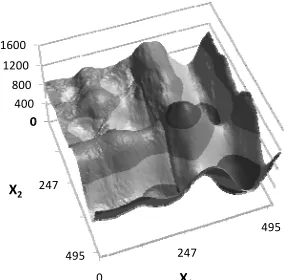
The ensembled and early-stopped plot of the Schwefel function, Fig. 2, does correctly map the global minimum and global maximum, but is clearly a poor approximation of Schwefel’s form (Fig. 1). The Langermann function, Fig. 3 likewise challenges the mapping ability of the CasCor neural network even with ensembling and early stopping (Fig. 4).

Some of the greatest strengths attributed to the CasCor type of neural network are as a result of it growing its own topology during training. An intrinsic feature is that at any point during training, no more than one new neuron will be having its weights optimised. Reputedly, this distinguishing behaviour results in rapid training times, however this is

challenged by [4], in which the authors also conclude that freezing of formerly trained weights can be detrimental to effective learning.

The universal function approximation abilities of the CasCor neural network, mathematically proven in [5], are only applicable if we assume that correct choices have been made when each and every neuron was inserted. By taking a system view of the training process, we argue that correct choices are not frequently made when mapping multimodal functions.

Figure 1 Schwefel function, range x(i) [0,500]

Figure 2 CasCor mapping of Schwefel with ensembling and early stopping

Informally, the training process plays the role of an agent in the system. This agent aims to train and fix in the network one neuron at a time that, in isolation, reduces the MSE on the training set by the largest possible amount. Several time steps later in the training, more neurons have been added and we see, with the benefit of hindsight, that incorrect choices have been made in the early stages of training. What were once apparently optimal additions to the network are ultimately conspiring to deflect the network from a good mapping of the underlying function. The training algorithm dictates that once neurons have been placed in the network, they may not be removed or re-trained (weight freezing) and so the problem becomes irreconcilable [4].

The problem has become one of decision theory – specifically evidential decision theory: how can a training process place a neuron in the network which, later in time, will combine with downstream neurons in only a beneficial way?

A more formal description can be found in [6] where they consider the problems caused when training on the simple “double-tanh” function. The problem is seen to be sufficient

0

247

495 0

400 800 1200 1600

0

247

495

X1

X2

0

247

495 0

400 800 1200 1600

0

247

495

X1

to preclude, or at least delay, convergence of the CasCor network.

In our training experiments with datasets that contain highly multimodal functions (Table I), the problem becomes clearer when monitoring the validation MSE. As the network is training, the insertion of new neurons should be conferring a greater information capacity to the neural network, and this MSE should decrease. Inserting the first two or three hidden neurons does cause a small decrease in the validation MSE but, soon after, this error increases resulting in a very poor generalization of the underlying function.

Figure 3 Langermann function, range x(i) [0,2]

Figure 4 CasCor mapping of Langermann with ensembling and early stopping

The hypothesis behind patchworking is that by subdividing the input domain, the number of extrema that any one neural network must approximate is kept below the multimodal threshold. Hence, CasCor networks with of a small number of neurons can wholly approximate the function over each subdivision with a lower MSE. In this way, patchworking overcomes the problems associated with weight freezing. Ensembling and early stopping can be used in conjunction with patchworking, and are in fact logical accompaniments.

Figure 5 Patchworking subdivisions for a 2D function

The technique is shown in Fig. 5 and is applied as follows: Subdivide the input domain so that no single neural network is required to map more than six extrema. Train further networks on the remaining subdivisions. This collection of networks we shall call a “patchwork” from visual similarity to that of a patchwork quilt. A relatively simple algorithm can be constructed to query such a patchwork, assuming that we have stored on file the minimum and maximum bounds of each network’s domain. Our patchworking algorithm is shown in the Appendix.

III. EXPERIMENTAL SET UP

The architecture of the CasCor algorithm is well known [1],[2],[7]. The CasCor neural networks under consideration are created from the open source library created by Nissen [8]. The library contains an implementation of the Cascade Correlation II algorithm based on the original Lisp code written by Fahlman in 1996 (unpublished).

Here, the FANN C source code is used with default settings chosen for CasCor training. The target MSE for the training is 10 when early stopping is not used and an arbitrary setting of 10 when early stopping is used. In use, the lower target will never be reached, due to early stopping

Table I Multimodal test functions

Function Name Range

De Jong’s 5th

0.002

where

32 16 0 16 32 32 … 0 16 32

32 32 32 32 32 16 … 32 32 32

20 20

1,2 (1)

Langermann 1 cos

0 2

1,2 ₍₂₎

Michalewicz sin · sin · 0 (3)

Schwefel 418.9829 sin 0 500 (4)

Shubert cos 1 cos 1 8 _1,2 6.2 (5)

Six Hump Camel Back 4 2.1 · 4 4 · 1.9 _{1 1} 1.9 (6)

0.0

1.0

2.0 ‐1

0 1

0.0

1.0

2.0

X1

X2

0.0

1.0

2.0 ‐1

0 1

0.0

1.0

2.0

X1

X2

triggering a halt to the training. The current release, 2.1.0-Beta, does not yet provide a neural network copy utility or functions that correctly scale and de-scale datasets, and so these have been added to our implementation.

A. Sampling and infill criteria

Orthogonal arrays (OAs) were chosen to sample our multimodal test functions. An OA is defined in the form

. . . . indicating an orthogonal array with runs, factors, levels, and strength . This is an array of size by , with entries from 0 to 1 with the property that in any columns you see each of the possibilities equally often [9]. The training set is made up from repeated runs of a trimmed version of . 25.6.5.2 [10]. With 25 evaluations being made each time, 20 runs of this OA are necessary to generate a training dataset of 500 points. The selection of the factors in each subsequent OA is known as the infill criteria, [11]: When subsequent OAs are evaluated, each of its factors are chosen to be those numerically furthest from all previously used factors.

The use of orthogonal arrays in the current work is only an artifact of the downstream application of this work in surrogate modelling, and their inclusion is not believed to alter the findings of this paper. In creating training datasets, less complex sampling methods should be sufficient to repeat our results.

B. Scaling

The range of all inputs and outputs is normalized to the interval [0.1,0.9] with the scaling factors saved after processing. These factors are later used to scale down the queries and scale up the neural network responses.

Note: All MSE errors presented in this paper are calculated on scaled data [0.1,0.9], thus making possible fair comparisons between otherwise disparate function output ranges.

C. Early stopping

For this work, we chose the size of the validation set as 30% of the size of the training set. Code from Beachkofski and Grandhi [12] provides the method of distributing the samples in the validation set. This “improved Latin hypercube” sampling was chosen because:

1) Generating validation sets of less than 1000 points is not computationally expensive and can be done at run time, 2) The algorithm in [12] produces points that fill the

hypercube uniformly, the statistical properties of which are desirable as described in [11],

3) The technique is fundamentally different from that used to generate the training set - ensuring that most, if not all, of the validation data points are automatically independent from those in the training set.

After the validation error is initialized to 1.0, our heuristic algorithm for early stopping is run each time a new hidden neuron is added to the network, and is given below:

• Test the network against the validation set

• If this new validation error is less than the old one, update the old validation error with this new value and make a copy of this “best network so far”.

• There must be at least five hidden neurons before early stopping can be initiated

• Early stopping can be applied retrospectively i.e. the best

network may end up having only four hidden neurons

• Early stopping is triggered on the earliest of:

o The error on the validation set becoming less than

5 10 (suitably low error)

o The validation error growing to be 50% larger than the smallest experienced validation error (network is diverging)

o More than 31 hidden neurons existing in the network (likelihood of a diverging network)

• When early stopping occurs, the “best network so far” is recalled from memory to replace the active network. The training is halted and the network is saved to permanent storage. The saved neural network will be that which had the smallest validation error.

D. Ensembling

When preparing an ensemble we need to answer the question of how many neural networks to include in that ensemble. Others have chosen an arbitrary number [3],[13] for their ensembles, but we investigated the ensemble size with respect to its influence on reducing the MSE.

Ensembles of CasCor neural networks were trained on the datasets, each test was repeated ten times for the larger ensembles and 30 times for ensembles smaller than ten. E. Patchworking

Fig. 10 shows the algorithm used to construct the patchwork. It allows for a user defined number of subdivisions known as “depth” and can be applied to as many input dimensions as is practical. Note, though, that the number of required networks grows exponentially

2 and so this method may not be practical if the dimensions number more than nine or ten. For two dimensional functions, an appropriate amount of training data per network (or “per patch”) was found to be between 25 and 70 samples per input dimension, hence, with four patches we used a training set of (size=500).

F. Testing the fit

One traditional test for the quality of regression fits (such as presented here) is to calculate the MSE against a testing set, in which the samples differ from those in the training set. Lower is better and so we can measure the success of the techniques herein by how much they reduce the MSE. The testing set is generated from the same algorithm as used for the validation sets [12], however it is larger. The size is chosen as 1000 where is the number of inputs to the neural network (or dimensions). The positioning of so many points is computationally expensive, especially when trying to maintain space filling properties. For this reason only one template is generated for all the testing sets (size=2000 queries).

IV. RESULTS A. Early stopping

B. Ensembling

To avoid losing clarity, only three of the six test functions are shown in Fig. 6, however, the form of the line graphs were similar throughout all six functions; the MSE reduced rapidly as the ensemble size increased from one to seven. Smaller reductions in the MSE occurred until ensembles greater than (size=25) were seen to deliver little or no benefit. We also used early stopping in this experiment and so the MSE’s in Fig. 6 reflect the combination of both techniques.

Figure 6 Reduction in mean squared error due to ensembling

The curves in Fig. 6 take the form:

(7)

Where is the MSE of a given neural network when ensembling is not used (Ens 1, and is the asymptote to which the curve tends. Effectively, represents an MSE boundary that no size of ensemble can reduce. By inspection of (7), larger ensemble sizes will be beneficial in reducing the MSE when β . Nevertheless, ensembling larger than 25 delivers too little benefit to be of practical use.

In Fig. 7 only the Michalewicz data is presented over a

smaller range of ensemble size. On this scatter graph, the Michalewicz MSE’s are represented as points. The line of best fit is (7) when =0.0117 and = 0.0060. Values of

and were found by linear regression.

Figure 7 Michalewicz scatter plot and the curve predicted by (7)

C. Patchworking

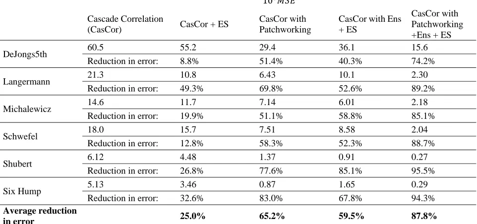
In Table II and Table III, Ens 15 is used. In Table II, the basic CasCor results are shown alongside the benefits of early stopping, patchworking, ensembling + early stopping, and all three combined. Patchworking is applied to (depth=1) and so the dataset is divided into four quarters. The same computer program was used to generate all the neural networks, the only changes being flags that turn on/off the features shown. Results shown are formed from the arithmetic mean of ten trials.

When compared to a standalone CasCor neural network, the effect of patchworking reduces the error an average of 3.3 times. Employing ensembling and early stopping on these functions reduces the error by an average factor of 3.0. However, the real benefit of patchworking is that it can be combined with the techniques of early stopping and ensembling – here delivering an average of an 11.3 times reduction in neural network testing error (87.8% reduction). D. Neurons added during training

Table III shows the average over ten repetitions of the

Table II Benefits of ES, Ens and, patchworking

10

Cascade Correlation

(CasCor) CasCor + ES

CasCor with Patchworking

CasCor with Ens + ES

CasCor with Patchworking +Ens + ES

DeJongs5th 60.5 55.2 29.4 36.1 15.6

Reduction in error: 8.8% 51.4% 40.3% 74.2%

Langermann 21.3 10.8 6.43 10.1 2.30

Reduction in error: 49.3% 69.8% 52.6% 89.2%

Michalewicz 14.6 11.7 7.14 6.01 2.18

Reduction in error: 19.9% 51.1% 58.8% 85.1%

Schwefel 18.0 15.7 7.51 8.58 2.04

Reduction in error: 12.8% 58.3% 52.3% 88.7%

Shubert 6.12 4.48 1.37 0.91 0.27

Reduction in error: 26.8% 77.6% 85.1% 95.5%

Six Hump 5.13 3.46 0.87 1.65 0.29

Reduction in error: 32.6% 83.0% 67.8% 94.3%

Average reduction

in error 25.0% 65.2% 59.5% 87.8%

0.000 0.002 0.004 0.006 0.008 0.010 0.012 0.014

0 10 20 30 40 50 60 70 80 90 100

M S E

Ensemble Size

Shubert

Michalewicz

Six Hump _0.000

0.002 0.004 0.006 0.008 0.010 0.012 0.014

0 5 10 15 20 25

M S E

Ensemble Size

((a‐b)/Ens_size)+b

number of neurons added during training. With no early stopping algorithm, several of the basic CasCor neural networks grow until they are stopped by an upper limit of the training (total_neurons < 35). Although a large number of neurons should confer a large information capacity, the high MSE’s in Table II show how poorly the basic CasCor networks map the multimodal functions.

The CasCor + Patchworking neuron count is smaller per network than the basic CasCor. The total_neuron limit is not causing termination of the training. The subdivision of the domain has meant that the training algorithm now ends either because the multimodal functions have been mapped successfully to the user specified MSE, or, the depth limit was reached. Since four networks are employed in the patchworked solutions, the information capacity of the patchwork is raised approximately four times. The reduced MSE’s for the patchwork solutions in Table II are a direct result of this greater capacity.

As would be expected, almost all of the CasCor with Ens + ES and the CasCor with Patchwork + Ens + ES results have lower neuron counts due to the early stopping mechanism halting the growth of each network. The low testing errors in Table II also reflect the improvements that ensembling delivers. The lowest errors are seen when all three techniques are combined; Ens, ES and patchworking each addressing the bias/variance, and information capacity problems of the CasCor neural network.

Table III Average number of neurons in each subdivision network

Cas- Cor

CasCor with Patchworking

CasCor with Ens + ES

CasCor with Patchworking +Ens + ES

De Jong’s

fifth 34 20.2 12.7 10.9 Langermann 34 16.6 13.9 10.1 Michalewicz 33.4 15.8 12.7 10.5

Schwefel 33 16.8 14.4 10.5

Shubert 29.9 12.4 15.0 10.5

Six Hump 29.3 12.4 14.9 10.8

E. Training time

Training times for the Schwefel function were 33s for the basic CasCor and 345s for the CasCor + Ens + ES; the larger time due to the cost of training the 15 ensemble elements. When patchworking alone was used, the time was 16s. With patchworking + Ens + ES the time was 168s. Of note is that patchworking has halved the training times of the comparable non-patchworked solutions. Despite the demand to train four times as many neural networks, the subdivision process has meant that each patch trains on a quarter of the 500 element training set – hence the reduced training times. The CPU was an Athlon 64 X2 2GHz with 512KB cache.

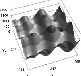
F. Visualization of patchworking + Ens + ES results Figs. 8 and 9 show clearly the significant improvement achieved by patchworking when compared to Figs. 2 and 4.

Figure 8 CasCor mapping of Schwefel (Patchworking + Ens + ES)

Figure 9 CasCor mapping of Langermann (Patchworking + Ens + ES)

V. CONCLUSION

All six functions presented here challenge the mapping capabilities of cascade correlation neural networks. Some redress is provided by early stopping and ensembling techniques; however, our results show that cascade correlation neural networks have an intrinsic weakness when presented with multimodal functions.

We introduced patchworking to subdivide the input domain and found a 3.3 times reduction in the mean squared error when used alone, and an 11.3 times improvement when used with ensembling and early stopping techniques. The patchworked solutions were found to have approximately half the training cost of non-patchworked solutions.

Further analysis of these results is planned, which will establish if the ensemble finding, (7), extends to other types of neural network. Investigating the size of the training datasets, with respect to its influence on the MSE, also warrants further investigation.

Variants of the CasCor neural network include one that only adds neurons to a single hidden layer (breadth) [2] and one that chooses whether to add depth or breadth to the network [14]. Both have mixed success against the standard CasCor. Lastly, Adams and Waugh [15] propose the open question of a two-stage training procedure. This type of training could keep most of CasCor’s speed benefits without the detrimental effects of weight freezing.

0

247

495 0

400 800 1200 1600

0

247

495

X1

X2

0.0

1.0

2.0 ‐1

0 1

0.0

1.0

2.0

X1

APPENDIX

Figure 10 The Patchworking algorithm

ACKNOWLEDGMENT

The authors are grateful to Adeline Schmitz of California State University for a discussion about her ensembling/early stopping experiments with the cascade correlation neural network, and, Steffen Nissen for creating and sharing FANN. Mike Riley thanks Rick G. Drury for his comments on early versions of this paper.

REFERENCES

[1] S. E. Fahlman and C. Lebiere, “The cascade-correlation learning architecture,” National Science Foundation under Contract Number EET-8716324 and Defense Advanced Research Projects Agency (DOD), ARPA Order No. 4976 under Contract F33615-87-C-1499., 1991.

[2] L. Prechelt, “Investigation of the cascor family of learning algorithms,” Neural Networks, vol. 10, pp. 885–896, 1996. [3] I. V. Tetko and A. E. P. Villa, “An enhancement of generalization

ability in cascade correlation algorithm by avoidance of overfitting/overtraining problem,” Neural Processing Letters, no. 6, pp. 43–50, 1997.

[4] C. S. Squires, Jr., and J. W. Shavlik, “Experimental analysis of aspects of the cascade-correlation learning architecture,” Computer Sciences Department, University of Wisconsin-Madison, Tech. Rep., 1991.

[5] T.Y. Kwok and D.Y. Yeung, “Objective functions for training new hidden units in constructive neural networks,” IEEE Transactions on Neural Networks, vol. 8, no. 5, pp. 1131–1148, Sep 1997.

[6] G. P. Drago and S. Ridella, “On the convergence of a growing topology neural algorithm,” Neurocomputing, vol. 12, no. 2-3, pp. 171–185, 1996.

[7] K. Mehrotra and S. Ranka, Elements of artificial neural networks. The MIT Press, 1996.

[8] FANN, http://leenissen.dk/fann/. Fast Artificial Neural Network Library. (Retrieved Jan 12th 2010.)

[9] N. J. A. Sloane, http://www2.research.att.com/ njas/oadir/. A Library of Orthogonal Arrays. (Retrieved Feb 8th 2010.) [10] W. F. Kuhfeld, http://support.sas.com/techsup/technote/ts723.html.

Orthogonal Arrays Provided as a Service of SAS (Retrieved Feb 8th 2010).

[11] A. Forrester, A. Sobester, and A. Keane, Engineering Design Via Surrogate Modelling: A Practical Guide. Wiley Blackwell, 2008. [12] B. Beachkofski and R. Grandhi, “Improved distributed hypercube

sampling,” in 43rd Structures, Structural Dynamics, and Materials Conference, 2002.

[13] A. Schmitz and H. Hefazi, “Constructive neural network ensemble for regression tasks in high dimensional spaces,” Sixth International Conference on Machine Learning and Applications, pp. 266–273, 2007.

[14] S. Baluja and S. E. Fahlman, “Reducing network depth in the cascade-correlation learning architecture,” Carnegie Mellon University, School of Computer Science, Tech. Rep., 1994. [15] A. Adams and S. Waugh, “Function evaluation and the