Learning Connective based Word Representations for Implicit Discourse Relation Identification

Learning Connective-based Word Representations

for Implicit Discourse Relation Identification

Chlo´e Braud

CoAStaL, Dep of Computer Science University of Copenhagen

University Park 5, 2100 Copenhagen, Denmark [email protected]

Pascal Denis

Magnet Team, INRIA Lille – Nord Europe 59650 Villeneuve dAscq, France

[email protected]

Abstract

We introduce a simple semi-supervised ap-proach to improve implicit discourse relation identification. This approach harnesses large amounts of automatically extracted discourse connectives along with their arguments to con-struct new distributional word representations. Specifically, we represent words in the space of discourse connectives as a way to directly encode their rhetorical function. Experiments on the Penn Discourse Treebank demonstrate the effectiveness of these task-tailored repsentations in predicting implicit discourse re-lations. Our results indeed show that, despite their simplicity, these connective-based rep-resentations outperform various off-the-shelf word embeddings, and achieve state-of-the-art performance on this problem.

1 Introduction

A natural distinction is often made between ex-plicit and imex-plicit discourse relations depending on whether they are lexicalized by a connective or not, respectively. To illustrate, the Contrast relation in example (1a) is triggered by the connective but, while it is not overtly marked in example (1b).1

Given the lack of strong explicit cues, the identi-fication of implicit relations is a much more chal-lenging and still open problem. The typically low performance scores for this task also hinder the de-velopment of text-level discourse parsers (Lin et al., 2010; Xue et al., 2015): implicit discourse relations 1_{These examples are taken from documents wsj 0008 and}

wsj 0037, respectively, of the PDTB.

account for around half of the data for different gen-res and languages (Prasad et al., 2008; Sporleder and Lascarides, 2008; Taboada, 2006; Subba and Di Eu-genio, 2009; Soria and Ferrari, 1998; Versley and Gastel, 2013).

(1) a. The house has voted to raise the ceiling to $3.1 trillion, but the Senate isn’t expected to act until next week at the earliest.

b. That’s not to say that the nutty plot of “A Wild Sheep Chase” is rooted in reality. It’s imaginative and often funny.

The difficulty of this task lies in its dependence on a wide variety of linguistic factors, ranging from syntax, lexical semantics and also world knowl-edge (Asher and Lascarides, 2003). In order to deal with this issue, a common approach is to exploit hand-crafted resources to design features captur-ing lexical, temporal, modal, or syntactic informa-tion (Pitler et al., 2009; Park and Cardie, 2012). By contrast, more recent work show that using simple low-dimensional word-based representations, either cluster-based or distributed (aka word embeddings), yield comparable or better performance (Rutherford and Xue, 2014; Braud and Denis, 2015), while dis-pensing with feature engineering.

While standard low-dimensional word represen-tations appear to encode relevant linguistic infor-mation, they have not been built with the specific rhetorical task in mind. A natural question is there-fore whether one could improve implicit discourse relation identification by using word representations that are more directly related to the task. The

problem of learning good representation for dis-course has been recently tackled by Ji and Eisen-stein (2014) on the problem of text-level discourse parsing. Their approach uses two recursive neural networks to jointly learn the task and a transforma-tion of the discourse segments to be attached. While this type of joint learning yields encouraging results, it is also computationally intensive, requiring long training times, and could be limited by the relatively small amount of manually annotated data available.

In this paper, we explore the possibility of learn-ing a distributional word representation adapted to the task by selecting relevant rhetorical contexts, in this case discourse connectives, extracted from large amounts of automatically detected connectives along with their arguments. Informally, the as-sumption is that the estimated word-connective co-occurrence statistics will in effect give us an im-portant insight to the rhetorical function of different words. The learning phase in this case is extremely simple, as it amounts to merely estimating co-occurrence frequencies, potentially combined with a reweighting scheme, between each word appearing in a discourse segment and its co-occurring connec-tive. To assess the usefulness of these connective-based representations,2 _{we compare them with}

pre-trained word representations, like Brown clusters and other word embeddings, on the task of implicit discourse relation identification. Our experiments on the Penn Discourse Treebank (PDTB) (Prasad et al., 2008) show that these new representations de-liver improvements over systems using these generic representations and yield state-of-the-art results, and this without the use of other hand-crafted features, thus also alleviating the need for external linguis-tic resources (like lexical databases). Thus, our ap-proach could be easily extended to resource-poor languages as long as connectives can be reliably identified on raw texts.

Section 2 summarizes related work. In Section 3, we detail our connective-based distributional word representation approach. Section 4 presents the au-tomatic annotation of the explicit examples used to build the word representation. In Section 5, we de-scribe our comparative experiments on the PDTB.

2_{Available at https://bitbucket.org/chloebt/} discourse-data.

2 Related Work

Implicit discourse relation identification has at-tracted growing attention since the release of the PDTB, the first discourse corpus to make the distinc-tion between explicit and implicit examples. Within the large body of research on this problem, we iden-tify two main strands directly relevant to our work.

2.1 Finding the Right Input Representation

The first work on this task (Marcu and Echihabi, 2002), which pre-dates the release of the PDTB, pro-posed a simple word-based representation: they use the Cartesian product of words appearing in the two segments. Given the knowledge-rich nature of the task, following studies attempted to exploit various hand-crafted resources and pre-processing systems to enrich their model with information on modality, polarity, tense, lexical semantics, and syntax, possi-bly combined with feature selection methods (Pitler et al., 2009; Lin et al., 2009; Park and Cardie, 2012; Biran and McKeown, 2013; Li and Nenkova, 2014). Interestingly, Park and Cardie (2012) con-cluded on the worthlessness of word-based features, as long as hand-crafted linguistic features were used. More recent studies however reversed this conclu-sion (Rutherford and Xue, 2014; Braud and Denis, 2015), demonstrating that word-based features can be effective provided they were not encoded using the sparse one-hot representation, but instead with a denser one (cluster based or distributed). This paper takes one step further by testing whether learning a simple task-specific, distributional word representa-tion could lead to further improvements.

2.2 Leveraging Explicit Discourse Data

Another line of work, also initiated in (Marcu and Echihabi, 2002), propose to deal with the sparseness of the word pair representation by using additional data automatically annotated using discourse con-nectives. An appeal of this strategy is that one can easily identify explicit relations in raw data, as per-formance are high on this task (Pitler et al., 2009) and it is even possible to rely on simple heuris-tics (Marcu and Echihabi, 2002; Sporleder and Las-carides, 2005; Lan et al., 2013). It has been shown, however, that using explicit examples as additional data for training an implicit relation classifier de-grades performance, due to important distribution differences (Sporleder and Lascarides, 2008).

Recent attempts to overcome this issue involve domain adaptation strategies (Braud and Denis, 2014; Ji et al., 2015), sample selection (Rutherford and Xue, 2015; Wang et al., 2012), or multi-task al-gorithms (Lan et al., 2013). However, it generally involves longer training time since models are built on a massive amount of data, the strategy requir-ing a large corpus of explicit examples to overcome the noise induced by the automatic annotation strat-egy. In this paper, we circumvent this problem by using explicit data only for learning our word repre-sentations and not for estimating the parameters of our implicit classification model. Some aspects of the present work are similar to Biran and McKeown (2013) in that they also exploit explicit data to com-pute co-occurrence statistics between word pairs and connectives. But the perspective is reversed, as they represent connectives in the contexts of co-occurring word pairs, with the aim of deriving similarity fea-tures between each implicit example and each con-nective. Furthermore, their approach did not outper-form state-of-the-art systems.

3 The Connective Vector Space Model Our discourse-based word representation model is a simple variant of the standard vector space model (Turney and Pantel, 2010): that is, it represents in-dividual words in specific co-occurring contexts (in this case, discourse connectives) that define the di-mensions of the underlying vector space. Our spe-cific choice of contexts was guided by two main con-siderations. On the one hand, we aim at learning

word representations that live in a relatively low-dimensional space, so as to make learning a classifi-cation function over that space feasible. The number of parameters of that function grows proportionally with that of the input size. Although there is often a lack of consensus among linguists as to the exact definition of discourse connectives, they neverthe-less form a closed class. For English, the PDTB rec-ognizes100distinct connectives. On the other hand, we want to learn a vectorial representation that cap-tures relevant aspects of the problem, in this case the rhetorical contribution of words. Adapting Har-ris (1954)’s famous quote, we make the assumption that words occurring in similarrhetorical contexts tend to have similarrhetoricalmeanings. Discourse connectives are by definition strong rhetorical cues. As an illustration, Pitler et al. (2009) found that con-nectives alone unambiguously predict a single rela-tion in94% of the PDTB level 1 data. By using

con-nectives as contexts, we are thus linking each word to a relation (or a small set of relations), namely those that can be triggered by this connective. Note that for level 2 relations in the PDTB, the connec-tives are much more ambiguous (86.77% reported in (Lin et al., 2010)), and it could be also the case if we expand the list of forms considered as connec-tives for English, or if we try to deal with other lan-guages and domains. We however believe that the set of relations that can be triggered by a connective is limited (not all relations can be expressed by the same connective), and that one attractive feature of our strategy is precisely to keep this ambiguity.

but while before

Word Freq. TF-IDF PPMI-IDF Freq. TF-IDF PPMI-IDF Freq. TF-IDF PPMI-IDF

reality 12 0.0 0.0 13 0.0 0.0 10 0.0 0.0

not 142 0.37 0.36 201 0.18 0.06 0 0.0 0.0

week 0 0.0 0.0 110 0.10 0.04 90 0.12 0.12

Table 1:Illustrative example of association measures between connectives and words.

3.1 Building the Distributional Representation

Our discourse-based representations of words are obtained by computing a matrix of co-occurrence between the words and the chosen contexts. The frequency counts are then weighted in order to high-light relevant associations. More formally, we note Vthe set of thenwords appearing in the arguments,

andCthe set of themconnective contexts. We build

the matrixF, of sizen_×m, by computing the fre-quency of each element ofV with each element of C. We notefi,j the frequency of the wordwi ∈ V

appearing in one argument of the connectivecj ∈ C.

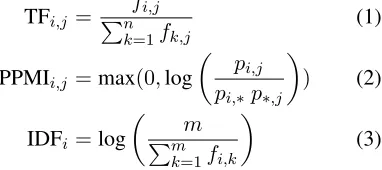
We use two standard weighting functions on these raw frequencies: the normalized Term Frequency (TF), eq. (1), and the Positive Pointwise Mutual In-formation (PPMI), eq. (2), which is a version of the PMI where negative values are ignored (with pi,j

the joint probability that the wordwi appears with

connective cj, and pi,∗ andp∗,j, relative frequency

of resp. wi andcj). These two measures are then

normalized by multiplying the value by the Inverse Document Frequency (IDF) for a word wi, eq. (3),

as in (Biran and McKeown, 2013). In the final ma-trices, theith_{row corresponds to them-dimensional}

vector for the ith word ofV. The jth column is a

vector corresponding to thejthconnective.

TFi,j = Pnfi,j

k=1fk,j (1)

PPMIi,j =max(0,log

pi,j pi,∗p∗,j

) (2)

IDFi=log

m Pm

k=1fi,k

(3)

Table 1 illustrates the weighting of the words using the TF and the PPMI normalized with IDF. For in-stance, the presence of the negation “not” is pos-itively linked to Contrast through but and while

whereas it receives a null or a very small weight with the temporal connectivebefore. The final

vec-tor for this word,< 0.37,0.18,0.0 >with TF-IDF

or< 0.36,0.06,0.0 >with PPMI-IDF, is intended

to guide the implicit model toward a contrastive lation, thus potentially helping in identifying the re-lation in example (1b). In contrast, the word “week” is more likely to be found in the arguments of tem-poral relations that can be triggered by before but alsowhile, an ambiguity kept in our representation whereas approaches based on using explicit exam-ples as new training data generally choose to anno-tate them using the most frequent sense associated with the connective, often limiting themselves to the less ambiguous ones (Marcu and Echihabi, 2002; Sporleder and Lascarides, 2008; Lan et al., 2013; Braud and Denis, 2014; Rutherford and Xue, 2015). Finally, a word occuring with all connectives, not discriminant, such as “reality” is associated with a null weight for all dimensions: it thus has no impact on the model.

Since we have100connectives for the PDTB, the representation is already of quite low dimensional-ity. However, it has been shown (Turney and Pan-tel, 2010) that using a dimensionality reduction al-gorithm could help capturing the latent dimensions between the words and their contexts and reducing the noise. We thus also test versions with a reduction Components Analysis (PCA) (Jolliffe, 2002).

3.2 Using the Word-based Representation

So far, our distributional framework associates a word with ad-dimensional vector (whered ≤ m).

ei-ther concatenating the two segment vectors (lead-ing to a 2d-dimensional vector) or by computing

the Kronecker product between them (leading to a d2-dimensional vector). Finally, these

segment-pair representations will be normalized using theL2

norm to avoid segment size effects. These will then be used as the input of a classification model, as described in Section 5. Given these combination schemes, it should be clear that despite the fact that each individual word receives a unique vectorial rep-resentation irrespective of its position, the param-eters of the classification model associated with a given word are likely to be different depending of whether it appears in the left or right segment.

4 Automatic Annotation of Explicit Examples

In order to collect reliable word-connective co-occurrence frequencies, we need a large corpus where the connectives and their arguments have been identified. We therefore rely on automatic annotation of raw data, instead of using the rela-tively small amount of explicit examples manually annotated in the PDTB (roughly18,000examples).

Specifically, we used the Bllip corpus3 _composed

of news articles from theLA Times, theWashington Post, theNew York TimesandReutersand containing

310millions of words automatically POS-tagged.

Identifying the Connectives and their Arguments

We have two tasks to perform: identifying the con-nectives and extracting their arguments.4 _Rather

than relying on manually defined patterns to anno-tate explicit examples (Marcu and Echihabi, 2002; Sporleder and Lascarides, 2008; Rutherford and Xue, 2015), we use two binary classification models inspired by previous works on the PDTB (Pitler and Nenkova, 2009; Lin et al., 2010): the first one iden-tifies the connectives and the second one localizes the arguments between inter- and intra-sentential, an heuristic being then used to decide on the exact boundaries of the arguments.

Discourse connectives are words (e.g.,but,since)

3_{https://catalog.ldc.upenn.edu/} LDC2008T13

4_{Note that contrary to studies using automatically annotated}

explicit examples as new training data, we do not need to anno-tate the relation triggered by the connective.

or grammaticalized multi-word expressions (e.g.,as soon as,on the other hand) that may trigger a dis-course relation. However, these forms can also ap-pear without any discourse reading, such asbecause

in: He can’t sleep because of the deadline. We thus need to disambiguate these forms between discourse and non discourse readings, a task that has proven to be quite easy on the PDTB (Pitler and Nenkova, 2009). This is the task performed by our first binary classifier: a pattern-matching is used to identify all potential connectives, and the model predicts if they have discourse reading in context.

We then need to extract the arguments of the iden-tified connectives, that is the two spans of text linked by the connective. This latter task has proven to be extremely hard on the PDTB (Lin et al., 2010; Xue et al., 2015) because of some annotation principles that make the possible types of argument very di-verse. As first proposed in (Lin et al., 2010), we thus split this task into two subtasks: identifying the rel-ative positions of the arguments and delimiting their exact boundaries.

For an explicit example in the PDTB, one argu-ment, calledArg2, is linked to the connective, and thus considered as easy to extract (Lin et al., 2010). The other argument, calledArg1, may be located at different places relative toArg2(Prasad et al., 2008): we call intra-sentential the examples whereArg1is a clause within the same sentence as Arg2 (60.9%

of the explicit examples in the PDTB), and inter-sentential the other examples, that isArg1 is found in the previous sentence, in a non-adjacent previ-ous sentence (9%) or in a following sentence (less than 0.1%). In this work, we build a localization

model by only considering these two coarse cases – the example is either intra- or inter-sentential. Note that this distinction is similar to what has been done in (Lin et al., 2010): more precisely, these authors distinguish between “same-sentence” and “previous sentence” and ignore the cases where theArg1is in a following sentence. We rather choose to include them as being also inter-sentential. When the posi-tion of Arg1 has been predicted, an heuristic is in charge of finding the exact boundaries of the argu-ments.

an argument can cover only a part of a sentence, an entire sentence or several sentences. Statistical ap-proaches intended to solve this task lead for now to low performance even when complex sequential models are used, and they often rely on the syntactic configurations (Lin et al., 2010; Xue et al., 2015). We thus decided to define an heuristic to perform this task, following the simplifying assumptions also used in previous work since (Marcu and Echihabi, 2002). We assume that: (1) Arg1 is either in the same sentence as Arg2 or in the previous one, (2) an argument covers at most one sentence and (3) a sentence contains at most two arguments. As it can be deduced from (1), our final model ignores the finer distinctions one can make for the position of inter-sentential examples (i.e. we never extractArg1

from a non-adjacent previous sentence or a follow-ing one).

According to these assumptions, once a connec-tive is identified, knowing its localization is almost enough to identify the boundaries of its arguments. More precisely, if a connective is predicted as inter-sentential, then our heuristic picks the entire pre-ceding sentence as Arg1, Arg2 being the sentence containing the connective, according to assumptions (1) and (2). If a connective is predicted as intra-sentential, then the sentence containing the connec-tive is split into two segments – according to (3) –, more precisely, the sentence is split around the con-nective using the punctuation and making it neces-sary to have a verb in each argument.

Settings We thus built two models using the PDTB: one to identify the discourse markers (con-nective vsnot connective), and one to identify the position of the arguments with respect to the con-nective (inter- vsintra-sentential). The PDTB con-tains18,459explicit examples for100connectives.

For both models, we use the same split of the data as in (Lin et al., 2014). The test set contains 923

positive instances of connectives and 2,075

nega-tive instances, and546inter-sentential and377

intra-sentential examples. Both models are built using a logistic regression model optimized on the develop-ment set (see Section 5), and the same simple feature set (Lin et al., 2014; Johannsen and Sgaard, 2013) without syntactic information. With C the connec-tive, F the following word and P the previous one,

our features are: C, P+C, C+F, C-POS5_{, P-POS,}

F-POS, P-POS+C-POS and C-POS+F-POS.

Results Our model identifies discourse connective with a micro-accuracy of92.9% (macro-F1 91.5%).

These scores are slightly lower than the state-of-the-art in micro-accuracy, but high enough to rely on this annotation. When applying our model to the

Bllipdata, we found4connectives that correspond

to no examples. We thus have examples for only96

connectives. For distinguishing between inter- and intra-sentential examples, we get a micro-accuracy of96.1% (macro-F196.0), with an F1of96.7for the

intra- and 95.3 for the inter-sentential class, again

close enough to the state-of-the-art (Lin et al., 2014).

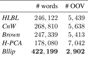
Coverage Using these models on Bllip, we are able to extract around3 million connectives, along

with their arguments. Our word representation has a large vocabulary (see Table 2) compared to exist-ing off-the-shelf word vectors, with only2,902out

of vocabulary (OOV) tokens in set of implicit rela-tions.6

# words # OOV

HLBL 246,122 5,439 CnW 268,810 5,638 Brown 247,339 5,413 H-PCA 178,080 7,042 Bllip 422,199 2,902

Table 2: Lexicon coverage forBrownclusters (Brown et al., 1992), Collobert and Weston (CnW) (Collobert and Weston, 2008) and hierarchical log-bilinear embeddings (HLBL) (Mnih and Hinton, 2007) using the implementation in (Turian et al., 2010), Hellinger PCA (H-PCA) (Lebret and Collobert, 2014) and our connective-based representation (Bllip).

5 Experiments

Our experiments investigate the relevance of our connective-based representations for implicit dis-course relation identification, recast here as multi-class multi-classification problem. That is, we aim at eval-uating the usefulness of having a word representa-tion linked to the task, compared to using generic 5_{The connective POS is either the node covering the}

con-nective, or the POS of its first word if no such node exists.

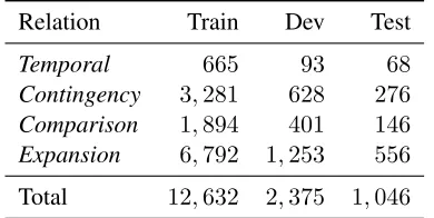
Relation Train Dev Test

Temporal 665 93 68

Contingency 3,281 628 276

Comparison 1,894 401 146

Expansion 6,792 1,253 556

Total 12,632 2,375 1,046 Table 3:Number of examples in train, dev, test.

word representations (either one-hot, cluster-based or distributed), and whether they encode all the in-formation relevant to the task, thus comparing sys-tems with or without additional hand-crafted fea-tures.

5.1 Data

The PDTB (Prasad et al., 2008) is the largest corpus annotated for discourse relations, formed by news-paper articles from the Wall Street Journal. It con-tains 16,053pairs of spans of text annotated with

one or more implicit relations. The relation set is organized in a three-level hierarchy. We focus on the level 1 coarse-grained relations and keep only the first relation annotated. We use the most spread split of the data, used in (Rutherford and Xue, 2014; Rutherford and Xue, 2015; Braud and Denis, 2015) among others, that is sections 2-20 for training and 21-22 for testing. The other sections are used for de-velopment. The number of examples per relation is reported in Table 3. It can be seen that the dataset is highly imbalanced, with the relationExpansion ac-counting for more than50% of the examples.

5.2 Settings

Feature Set Our main features are based on the words occurring in the arguments. We test simple baselines using raw tokens. The first one uses the Cartesian product of the tokens, a feature template, generally called ”Word pairs”, used in most of the previous study for this task as in (Marcu and Echi-habi, 2002; Pitler et al., 2009; Lin et al., 2011; Braud and Denis, 2015; Ji et al., 2015). It is the sparsest representation one can build from words, and it cor-responds to using the combination scheme based on the Kronecker product to combine the one-hot vec-tors representing each word. We also report results with a less sparse version where the vectors are

com-bined using concatenation.

We also compare our systems to previous ap-proaches that make use of word based representa-tions but not linked to the task. We implement the systems proposed in (Braud and Denis, 2015) in multiclass, that is using theBrownclusters (Brown et al., 1992), the Collobert and Weston (Collobert and Weston, 2008) and the hierarchical log-bilinear embeddings (Mnih and Hinton, 2007) using the implementation in (Turian et al., 2010)7_{, and the} HPCA (Lebret and Collobert, 2014)8_{. We use}

the combination schemes described in Section 3 to build vector representations for pairs of segments. For these systems and ours, using the connective-based representations, the dimensionality of the final model depends on the number of dimensionsdof the

representation used and on the combination scheme – the concatenation leading to2ddimensions and the

Kronecker product tod2.

All the word representations used – the off-the-shelf representations as well as our connective-based representation (see Section 4) – are solely or mainly trained on newswire data, thus on the same domain as our evaluation data. The CnW embeddings we use in this paper, with the implementation in (Turian et al., 2010), as well as theHLBLembeddings have been obtained using the RCV1 corpus, that is one year of Reuters English newswire. TheH-PCAhave been built on the Wikipedia, the Reuters corpus and the Wall street Journal. We thus do not expect any out-of-domain issue when using these representa-tions.

Finally, we experiment with additional features proposed in previous studies and well described in (Pitler et al., 2009; Park and Cardie, 2012): pro-duction rules9_{, information on verbs (average verb}

phrases length and Levin classes), polarity (Wilson et al., 2005), General Inquirer tags (Stone and Kirsh, 1966), information about the presence of numbers and modals, and first, last and first three words. We concatenate these features to the ones built using word representations.

7_{http://metaoptimize.com/projects/} wordreprs/

8_{http://lebret.ch/words/}

9_{We use the gold standard parses provided in the Penn}

Model We train a multinomial multiclass logistic regression model.10 _{In order to deal with the class}

imbalance issue, we use a sample weighting scheme where each instance has a weight inversely propor-tional to the frequency of the class it belongs to.

Parameters We optimize the hyper-parameters of the algorithm, that is the regularization norm (L1 or L2), and the strength of the regularization C ∈ {0.001,0.005,0.01,0.1,0.5,1,5,10,100}. When using additional features or one-hot sparse encod-ings over the pairs of raw tokens, we also optimize a filter on the features by defining a frequency cut-off t _{∈ {}1,2,5,10,15,20_}. We evaluate the

un-supervised representations with different number of dimensions. We test versions of the Brown clus-ters with 100, 320, 1,000 and 3,200 clusters, of

the Collobert and Weston embeddings with25, 50,

100 and 200 dimensions, of the hierarchical

log-bilinear embeddings with 50 and 100 dimensions,

and of the Hellinger PCA with50,100and200 di-mensions. Finally, the distributional representations of words based on the connective are built using ei-ther no PCA – thus corresponding to96dimensions– , or a PCA11 _{keeping the first k dimensions with} k _{∈ {}2,5,10,50_}.12 We optimize both the

hyper-parameters of the algorithm and the number of di-mensions of the unsupervised representation on the development set based on the macro-F1 score, the

most relevant measure to track when dealing with imbalanced data.

5.3 Results

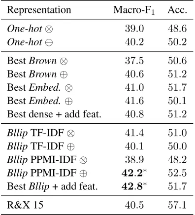
Our results are summarized in Table 4. Using our connective-based word representation allows im-provements of above2% in macro-F1over the

base-line systems based on raw tokens (One-hot), the competitive systems using pre-trained representa-tions (Brown and Embed.) and the state-of-the-art results in terms of macro-F1 (R&X 15). These

im-provements demonstrate the efficiency of the repre-sentation for this task.

We found that using an unsupervised word repre-sentation generally leads to improvements over the

10_{http://scikit-learn.org/dev/index.html.} 11_{Implemented in scikit-learn, applied with default settings.} 12_{Keeping resp.11.3%,36.6%,56.2% or95.3% of the}

vari-ance of the data.

Representation Macro-F1 Acc.

One-hot⊗ 39.0 48.6

One-hot⊕ 40.2 50.2

BestBrown⊗ 37.5 50.6

BestBrown⊕ 40.6 51.2

BestEmbed.⊗ 41.0 51.7

BestEmbed.⊕ 41.6 50.1

Best dense + add feat. 40.8 51.2 BllipTF-IDF⊗ 41.4 51.0 BllipTF-IDF⊕ 40.1 50.0 BllipPPMI-IDF⊗ 38.9 48.2 BllipPPMI-IDF⊕ 42.2∗ 52.5

BestBllip+ add feat. 42.8∗ 51.7

R&X 15 40.5 57.1 Table 4: Results for multiclass experiments. R&X 15 are the scores reported in (Rutherford and Xue, 2015) ;One-hot: one-hot encoding of raw tokens ;Brownand Embed.: pre-trained representations ;Bllip: connective based representation.∗_p≤

0.1compared toOne-hot⊗with t-test and Wilcoxon.

use of raw tokens (One-hot), a conclusion in line with the results reported in (Braud and Denis, 2015) for binary systems. However, contrary to their find-ings, in multiclass, the best results are not obtained using theBrownclusters, but rather the dense, real valued representations (Embed. andBllip). Further-more, concerning the combination schemes, the con-catenation (⊕) generally outperforms the Kronecker product (⊗), in effect favoring lower dimensional models.

2 5 10 25 50 100 200

25 30 35 40

Number of dimensions F1

on

the

de

v

set

Bllip PPMI⊕

CnW⊕

HLBL⊕

H-PCA⊕

Figure 1:F1scores on dev against the number of dimensions.

Our best results with Bllip are obtained without the use of a dimensionality reduction method, thus keeping the96dimensions corresponding to the

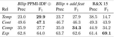
con-nectives identified in the raw data. Our new word representation like the other low-dimensional ones yield higher scores as one increases the number of dimensions (see Figure 1). This could be a limita-tion of our strategy, since the number of connectives in the PDTB is fixed. However, one could easily expand our model to include additional lexical ele-ments that might have a rhetorical function such as modals or specific expressions such asone reason is. We also tested the addition of hand-crafted fea-tures traditionally used for the task. We found that, either using a pre-trained word representation or our representation based on connectives, adding these features leads to small or even no improvements and suggest that these representations already encode the information provided by these features. This con-clusion has however to be nuanced: when looking at the scores per relation reported in Table 5, the use of the connective based word representation alone allows the best performance forTemporaland Con-tingency, but the addition of new features dramat-ically increase the scores for Comparisonshowing that some information are missing for this relation. Moreover, this relation is the one taking the most advantage of the addition of explicit data in (Ruther-ford and Xue, 2015), demonstrating that these data could probably provide even more information than the ones we leverage through our representations.

Finally, our results are similar or even better than those reported in (Rutherford and Xue, 2015) in terms of macro-F1. Our systems correspond

how-ever to a lower micro-accuracy. Looking at the scores per relation in Table 5, we found that we ob-tain better results for all the relations except Expan-sion, the most represented, which could explain the loss in accuracy. It is noteworthy that we generally obtain better results even without the additional fea-tures used in this work. Moreover, our systems re-quires lower training time (since we only train on implicit examples) and alleviate the need for the sample selection strategy used to deal with the dis-tribution differences between the two types of data.

BllipPPMI-IDF⊕ Bllip + add feat R&X 15

Rel Prec F1 Prec F1 Prec F1

Temp 23.0 29.9 23.7 27.9 38.5 14.7

Cont 49.6 47.1 46.7 46.3 49.3 43.9

Comp 35.9 27.7 35.0 34.3 44.9 34.2

Exp 62.8 64.0 63.7 62.6 61.4 69.1

Table 5:Scores per relation for multiclass experiments, ”R&X 15” are the scores reported in (Rutherford and Xue, 2015).

6 Conclusion

We presented a new approach to leverage infor-mation from explicit examples for implicit relation identification. We showed that building distribu-tional representations linked to the task through con-nectives allows state-of-the-art performance and al-leviates the need for additional features. Future work includes extending the representations to new contexts – such as the Alternative Lexicalization an-notated in the PDTB, the modals or some adverbs – using more sophisticated weighting schemes (Le-bret and Collobert, 2014) and testing this strategy for other languages and domains.

Acknowledgements

References

Nicholas Asher and Alex Lascarides. 2003. Logics of Conversation. Cambridge University Press.

Or Biran and Kathleen McKeown. 2013. Aggregated word pair features for implicit discourse relation dis-ambiguation. InProceedings of ACL.

Chlo´e Braud and Pascal Denis. 2014. Combining natural and artificial examples to improve implicit discourse relation identification. InProceedings of COLING. Chlo´e Braud and Pascal Denis. 2015. Comparing word

representations for implicit discourse relation classifi-cation. InProceedings of EMNLP.

Peter F. Brown, Peter V. deSouza, Robert L. Mercer, Vin-cent J. Della Pietra, and Jenifer C. Lai. 1992. Class-based n-gram models of natural language. Computa-tional Linguistics, 18:467–479.

Lynn Carlson, Daniel Marcu, and Mary Ellen Okurowski. 2001. Building a discourse-tagged corpus in the framework of rhetorical structure theory. In Proceed-ings of the Second SIGdial Workshop on Discourse and Dialogue.

Ronan Collobert and Jason Weston. 2008. A unified ar-chitecture for natural language processing: Deep neu-ral networks with multitask learning. InProceedings of ICML.

Juliette Conrath, Stergos Afantenos, Nicholas Asher, and Philippe Muller. 2014. Unsupervised extraction of se-mantic relations using discourse cues. InProceedings of Coling.

Zellig S. Harris. 1954. Distributional structure. Word, 10(23):146–162.

Yangfeng Ji and Jacob Eisenstein. 2014. Representation learning for text-level discourse parsing. In Proceed-ings of ACL.

Yangfeng Ji, Gongbo Zhang, and Jacob Eisenstein. 2015. Closing the gap: Domain adaptation from explicit to implicit discourse relations. In Proceedings of EMNLP.

Anders Johannsen and Anders Sgaard. 2013. Disam-biguating explicit discourse connectives without ora-cles. InProceedings of IJCNLP.

Ian Jolliffe. 2002. Principal component analysis. Wiley Online Library.

Man Lan, Yu Xu, and Zhengyu Niu. 2013. Leveraging synthetic discourse data via multi-task learning for im-plicit discourse relation recognition. InProceedings of ACL.

R´emi Lebret and Ronan Collobert. 2014. Word emded-dings through Hellinger PCA. InProceedings of ACL. Junyi Jessy Li and Ani Nenkova. 2014. Reducing spar-sity improves the recognition of implicit discourse re-lations. InProceedings of SIGDIAL.

Ziheng Lin, Min-Yen Kan, and Hwee Tou Ng. 2009. Recognizing implicit discourse relations in the Penn Discourse Treebank. InProceedings of EMNLP. Ziheng Lin, Hwee Tou Ng, and Min-Yen Kan. 2010. A

PDTB-styled end-to-end discourse parser. Technical report, National University of Singapore.

Ziheng Lin, Hwee Tou Ng, and Min-Yen Kan. 2011. Au-tomatically evaluating text coherence using discourse relations. InProceedings of ACL-HLT.

Ziheng Lin, Hwee Tou Ng, and Min-Yen Kan. 2014. A PDTB-styled end-to-end discourse parser. Natural Language Engineering, 20:151–184.

Daniel Marcu and Abdessamad Echihabi. 2002. An unsupervised approach to recognizing discourse rela-tions. InProceedings of ACL.

Mitchell P. Marcus, Beatrice Santorini, and Mary Ann Marcinkiewicz. 1993. Building a large annotated cor-pus of english: The Penn Treebank. Computational Linguistics, 19(2):313–330.

Andriy Mnih and Geoffrey Hinton. 2007. Three new graphical models for statistical language modelling. In

Proceedings of ICML.

Joonsuk Park and Claire Cardie. 2012. Improving im-plicit discourse relation recognition through feature set optimization. InProceedings of SIGDIAL Conference. Emily Pitler and Ani Nenkova. 2009. Using syntax to disambiguate explicit discourse connectives in text. In

Proceedings of the ACL-IJCNLP.

Emily Pitler, Annie Louis, and Ani Nenkova. 2009. Au-tomatic sense prediction for implicit discourse rela-tions in text. InProceedings of ACL-IJCNLP. Rashmi Prasad, Nikhil Dinesh, Alan Lee, Eleni

Milt-sakaki, Livio Robaldo, Aravind Joshi, and Bonnie Webber. 2008. The Penn Discourse Treebank 2.0. In

Proceedings of LREC.

Attapol Rutherford and Nianwen Xue. 2014. Discover-ing implicit discourse relations through Brown cluster pair representation and coreference patterns. In Pro-ceedings of EACL.

Attapol Rutherford and Nianwen Xue. 2015. Improving the inference of implicit discourse relations via classi-fying explicit discourse connectives. InProceedings of NAACL-HLT.

Claudia Soria and Giacomo Ferrari. 1998. Lexical mark-ing of discourse relations - some experimental find-ings. In Proceedings of the ACL Workshop on Dis-course Relations and DisDis-course Markers.

Caroline Sporleder and Alex Lascarides. 2005. Exploit-ing lExploit-inguistic cues to classify rhetorical relations. In

Proceedings of RANLP-05.

Philip J. Stone and John Kirsh. 1966. The General In-quirer: A Computer Approach to Content Analysis. MIT Press.

Rajen Subba and Barbara Di Eugenio. 2009. An effec-tive discourse parser that uses rich linguistic informa-tion. InProceedings of ACL-HLT.

Maite Taboada. 2006. Discourse markers as signals (or not) of rhetorical relations. Journal of Pragmatics, 38:567–592.

Joseph Turian, Lev-Arie Ratinov, and Yoshua Bengio. 2010. Word representations: A simple and general method for semi-supervised learning. InProceedings of ACL.

Peter D. Turney and Patrick Pantel. 2010. From fre-quency to meaning : Vector space models of seman-tics. Journal of Artificial Intelligence Research, pages 141–188.

Yannick Versley and Anna Gastel. 2013. Linguistic tests for discourse relations in the T¨uBa-D/Z corpus of writ-ten German. Dialogue & Discourse, 4(2):142–173. Xun Wang, Sujian Li, Jiwei Li, and Wenjie Li. 2012.

Im-plicit discourse relation recognition by selecting typ-ical training examples. In Proceedings of COLING 2012: Technical Papers.

Theresa Wilson, Janyce Wiebe, and Paul Hoffmann. 2005. Recognizing contextual polarity in phrase-level sentiment analysis. InProceedings of HLT-EMNLP. Nianwen Xue, Hwee Tou Ng, Sameer Pradhan, Rashmi