A Fast and Accurate Dependency Parser using Neural Networks

A Fast and Accurate Dependency Parser using Neural Networks

Danqi Chen

Computer Science Department Stanford University [email protected]

Christopher D. Manning Computer Science Department

Stanford University [email protected]

Abstract

Almost all current dependency parsers classify based on millions of sparse indi-cator features. Not only do these features generalize poorly, but the cost of feature computation restricts parsing speed signif-icantly. In this work, we propose a novel way of learning a neural network classifier for use in a greedy, transition-based depen-dency parser. Because this classifier learns and uses just a small number of dense fea-tures, it can work very fast, while achiev-ing an about 2% improvement in unla-beled and launla-beled attachment scores on both English and Chinese datasets. Con-cretely, our parser is able to parse more than 1000 sentences per second at 92.2% unlabeled attachment score on the English Penn Treebank.

1 Introduction

In recent years, enormous parsing success has been achieved by the use of feature-based discrim-inative dependency parsers (K¨ubler et al., 2009). In particular, for practical applications, the speed of the subclass of transition-based dependency parsers has been very appealing.

However, these parsers are not perfect. First, from a statistical perspective, these parsers suffer from the use of millions of mainly poorly esti-mated feature weights. While in aggregate both lexicalized features and higher-order interaction term features are very important in improving the performance of these systems, nevertheless, there is insufficient data to correctly weight most such features. For this reason, techniques for introduc-ing higher-support features such as word class fea-tures have also been very successful in improving parsing performance (Koo et al., 2008). Second, almost all existing parsers rely on a manually de-signed set of feature templates, which require a lot

of expertise and are usually incomplete. Third, the use of many feature templates cause a less stud-ied problem: in modern dependency parsers, most of the runtime is consumed not by the core pars-ing algorithm but in the feature extraction step (He et al., 2013). For instance, Bohnet (2010) reports that his baseline parser spends 99% of its time do-ing feature extraction, despite that bedo-ing done in standard efficient ways.

In this work, we address all of these problems by using dense features in place of the sparse indi-cator features. This is inspired by the recent suc-cess of distributed word representations in many NLP tasks, e.g., POS tagging (Collobert et al., 2011), machine translation (Devlin et al., 2014), and constituency parsing (Socher et al., 2013). Low-dimensional, dense word embeddings can ef-fectively alleviate sparsity by sharing statistical strength between similar words, and can provide us a good starting point to construct features of words and their interactions.

Nevertheless, there remain challenging prob-lems of how to encode all the available infor-mation from the configuration and how to model higher-order features based on the dense repre-sentations. In this paper, we train a neural net-work classifier to make parsing decisions within a transition-based dependency parser. The neu-ral network learns compact dense vector represen-tations of words, part-of-speech (POS) tags, and dependency labels. This results in a fast, com-pact classifier, which uses only 200 learned dense features while yielding good gains in parsing ac-curacy and speed on two languages (English and Chinese) and two different dependency represen-tations (CoNLL and Stanford dependencies). The main contributions of this work are: (i) showing the usefulness of dense representations that are learned within the parsing task, (ii) developing a neural network architecture that gives good accu-racy and speed, and (iii) introducing a novel

vation function for the neural network that better captures higher-order interaction features.

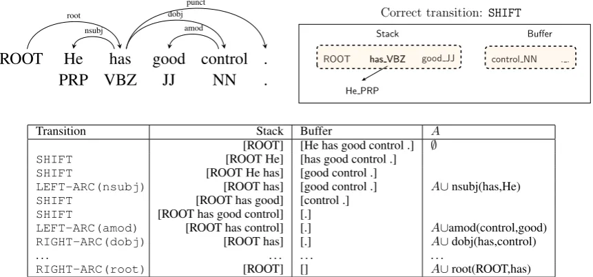
2 Transition-based Dependency Parsing Transition-based dependency parsing aims to pre-dict a transition sequence from an initial configu-ration to some terminal configuconfigu-ration, which de-rives a target dependency parse tree, as shown in Figure 1. In this paper, we examine only greedy parsing, which uses a classifier to predict the cor-rect transition based on features extracted from the configuration. This class of parsers is of great in-terest because of their efficiency, although they tend to perform slightly worse than the search-based parsers because of subsequent error prop-agation. However, our greedy parser can achieve comparable accuracy with a very good speed.1

As the basis of our parser, we employ the arc-standard system (Nivre, 2004), one of the most popular transition systems. In the arc-standard system, a configuration c = (s, b, A)

consists of a stack s, a buffer b, and a set of

dependency arcs A. The initial configuration for a sentence w1, . . . , wn is s = [ROOT], b =

[w1, . . . , wn], A = ∅. A configurationcis termi-nal if the buffer is empty and the stack contains the single nodeROOT, and the parse tree is given by Ac. Denoting si (i = 1,2, . . .) as the ith top element on the stack, andbi (i = 1,2, . . .)as the

ith _{element on the buffer, the arc-standard system}

defines three types of transitions:

• LEFT-ARC(l): adds an arc s1 → s2 with

labell and removess2 from the stack.

Pre-condition:|s| ≥2.

• RIGHT-ARC(l): adds an arcs2 → s1 with

labell and removess1 from the stack.

Pre-condition:|s| ≥2.

• SHIFT: moves b1 from the buffer to the

stack. Precondition:|b| ≥1.

In the labeled version of parsing, there are in total

|T | = 2Nl+ 1 transitions, where Nl is number of different arc labels. Figure 1 illustrates an ex-ample of one transition sequence from the initial configuration to a terminal one.

The essential goal of a greedy parser is to pre-dict a correct transition from T, based on one

1_{Additionally, our parser can be naturally incorporated} with beam search, but we leave this to future work.

Single-word features(9)

s1.w;s1.t;s1.wt;s2.w;s2.t;

s2.wt;b1.w;b1.t;b1.wt

Word-pair features(8)

s1.wt◦s2.wt;s1.wt◦s2.w;s1.wts2.t;

s1.w◦s2.wt;s1.t◦s2.wt;s1.w◦s2.w

s1.t◦s2.t;s1.t◦b1.t

Three-word feaures(8)

s2.t◦s1.t◦b1.t;s2.t◦s1.t◦lc1(s1).t;

s2.t◦s1.t◦rc1(s1).t;s2.t◦s1.t◦lc1(s2).t;

s2.t◦s1.t◦rc1(s2).t;s2.t◦s1.w◦rc1(s2).t;

s2.t◦s1.w◦lc1(s1).t;s2.t◦s1.w◦b1.t

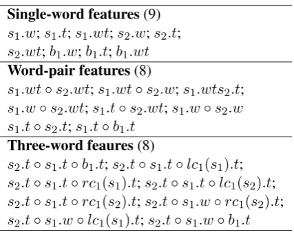
Table 1: The feature templates used for analysis.

lc1(si) andrc1(si) denote the leftmost and right-most children of si, w denotes word, t denotes POS tag.

given configuration. Information that can be ob-tained from one configuration includes: (1) all the words and their corresponding POS tags (e.g.,

has /VBZ); (2) the head of a word and its label (e.g., nsubj, dobj) if applicable; (3) the posi-tion of a word on the stack/buffer or whether it has already been removed from the stack.

Conventional approaches extract indicator fea-tures such as the conjunction of 1 ∼ 3 elements from the stack/buffer using their words, POS tags or arc labels. Table 1 lists a typical set of feature templates chosen from the ones of (Huang et al., 2009; Zhang and Nivre, 2011).2 _{These features}

suffer from the following problems:

• Sparsity. The features, especially lexicalized features are highly sparse, and this is a com-mon problem in many NLP tasks. The sit-uation is severe in dependency parsing, be-cause it depends critically on word-to-word interactions and thus the high-order features. To give a better understanding, we perform a feature analysis using the features in Table 1 on the English Penn Treebank (CoNLL rep-resentations). The results given in Table 2 demonstrate that: (1) lexicalized features are indispensable; (2) Not only are the word-pair features (especiallys1 ands2) vital for

pre-dictions, the three-word conjunctions (e.g.,

{s2, s1, b1}, {s2, lc1(s1), s1}) are also very

important.

ROOT He

has good control .

PRP VBZ

JJ

NN

.

root nsubj

punct dobj

amod

1

ROOT has VBZ

He PRP

nsubj

has VBZ good JJ control NN . .

Stack Bu↵er

Correct transition: SHIFT

1

Transition Stack Buffer A

[ROOT] [He has good control .] ∅

SHIFT [ROOT He] [has good control .]

SHIFT [ROOT He has] [good control .]

LEFT-ARC(nsubj) [ROOT has] [good control .] A∪nsubj(has,He)

SHIFT [ROOT has good] [control .]

SHIFT [ROOT has good control] [.]

LEFT-ARC(amod) [ROOT has control] [.] A∪amod(control,good)

RIGHT-ARC(dobj) [ROOT has] [.] A∪dobj(has,control)

. . . .

RIGHT-ARC(root) [ROOT] [] A∪root(ROOT,has)

Figure 1: An example of transition-based dependency parsing. Above left: a desired dependency tree, above right: an intermediate configuration, bottom: a transition sequence of the arc-standard system.

Features UAS

All features in Table 1 88.0 single-word & word-pair features 82.7 only single-word features 76.9 excluding all lexicalized features 81.5 Table 2: Performance of different feature sets. UAS: unlabeled attachment score.

• Incompleteness. Incompleteness is an un-avoidable issue in all existing feature tem-plates. Because even with expertise and man-ual handling involved, they still do not in-clude the conjunction of every useful word combination. For example, the conjunc-tion of s1 and b2 is omitted in almost all

commonly used feature templates, however it could indicate that we cannot perform a

RIGHT-ARCaction if there is an arc froms1

tob2.

• Expensive feature computation. The fea-ture generation of indicator feafea-tures is gen-erally expensive — we have to concatenate some words, POS tags, or arc labels for gen-erating feature strings, and look them up in a huge table containing several millions of fea-tures. In our experiments, more than95%of the time is consumed by feature computation during the parsing process.

So far, we have discussed preliminaries of

transition-based dependency parsing and existing problems of sparse indicator features. In the fol-lowing sections, we will elaborate our neural net-work model for learning dense features along with experimental evaluations that prove its efficiency.

3 Neural Network Based Parser

In this section, we first present our neural network model and its main components. Later, we give details of training and speedup of parsing process.

3.1 Model

Figure 2 describes our neural network architec-ture. First, as usual word embeddings, we repre-sent each word as ad-dimensional vectorew

i ∈Rd and the full embedding matrix is Ew _{∈ R}d×Nw

where Nw is the dictionary size. Meanwhile, we also map POS tags and arc labels to a d -dimensional vector space, whereet

i, elj ∈ Rdare the representations ofith _{POS tag andj}th _arc

la-bel. Correspondingly, the POS and label embed-ding matrices areEt _{∈ R}d×Nt andEl ∈ Rd×Nl

whereNt andNl are the number of distinct POS tags and arc labels.

· · · · · · · · · ·

Input layer: [xw_{, x}t_{, x}l_] Hidden layer:

h= (Ww

1 xw+W1txt+W1lxl+b1)3

Softmax layer:

p = softmax(W2h)

words POS tags arc labels

ROOT has VBZ

He PRPnsubj

has VBZ good JJ control NN . .

Stack Buffer

Configuration

Figure 2: Our neural network architecture.

{lc1(s2).t, s2.t, rc1(s2).t, s1.t}, we will extract

PRP,VBZ,NULL,JJin order. Here we use a spe-cial token NULL to represent a non-existent ele-ment.

We build a standard neural network with one hidden layer, where the corresponding embed-dings of our chosen elements fromSw_{, S}t_{, S}l_will be added to the input layer. Denotingnw, nt, nlas the number of chosen elements of each type, we addxw _{= [e}w

w1;eww2;. . . ewwnw]to the input layer,

where Sw _{= {w1, . . . , wn}

w}. Similarly, we add

the POS tag featuresxt_{and arc label featuresx}l_to the input layer.

We map the input layer to a hidden layer with

dhnodes through acube activation function:

h= (Ww

1 xw+W1txt+W1lxl+b1)3

where Ww

1 ∈ Rdh×(d·nw), W1t ∈ Rdh×(d·nt),

Wl

1 ∈Rdh×(d·nl), andb1∈Rdhis the bias.

A softmax layer is finally added on the top of the hidden layer for modeling multi-class prob-abilities p = softmax(W2h), where W2 ∈

R|T |×dh.

POS and label embeddings

To our best knowledge, this is the first attempt to introduce POS tag and arc label embeddings in-stead of discrete representations.

Although the POS tags P = {NN,NNP,

NNS,DT,JJ, . . .} (for English) and arc labels

L = {amod,tmod,nsubj,csubj,dobj, . . .}

(for Stanford Dependencies on English) are rela-tively small discrete sets, they still exhibit many semantical similarities like words. For example,

NN(singular noun) should be closer toNNS(plural

−1 −0.8 −0.6 −0.4 −0.2 0.2 0.4 0.6 0.8 1

−1 −0.5 0.5 1

cube sigmoid

tanh identity

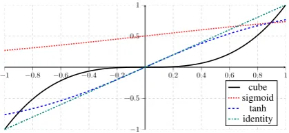
Figure 3: Different activation functions used in neural networks.

noun) thanDT(determiner), andamod(adjective modifier) should be closer tonum(numeric mod-ifier) than nsubj(nominal subject). We expect these semantic meanings to be effectively captured by the dense representations.

Cube activation function

As stated above, we introduce a novel activation function: cube g(x) = x3 _{in our model instead}

of the commonly used tanh or sigmoid functions (Figure 3).

Intuitively, every hidden unit is computed by a (non-linear) mapping on a weighted sum of input units plus a bias. Using g(x) = x3 _{can model}

the product terms ofxixjxkfor any three different elements at the input layer directly:

g(w1x1+. . .+wmxm+b) =

X

i,j,k

(wiwjwk)xixjxk+

X

i,j

b(wiwj)xixj. . .

ele-ments, which is a very desired property of depen-dency parsing.

Experimental results also verify the success of the cube activation function empirically (see more comparisons in Section 4). However, the expres-sive power of this activation function is still open to investigate theoretically.

The choice ofSw_{, S}t_{, S}l

Following (Zhang and Nivre, 2011), we pick a rich set of elements for our final parser. In de-tail,Sw_{containsnw = 18elements: (1) The top 3} words on the stack and buffer:s1, s2, s3, b1, b2, b3;

(2) The first and second leftmost / rightmost children of the top two words on the stack:

lc1(si), rc1(si), lc2(si), rc2(si), i = 1,2. (3) The leftmost of leftmost / rightmost of right-most children of the top two words on the stack:

lc1(lc1(si)), rc1(rc1(si)),i= 1,2.

We use the corresponding POS tags for St (nt = 18), and the corresponding arc labels of words excluding those 6 words on the stack/buffer forSl(nl = 12). A good advantage of our parser is that we can add a rich set of elements cheaply, instead of hand-crafting many more indicator fea-tures.

3.2 Training

We first generate training examples {(ci, ti)}mi=1

from the training sentences and their gold parse trees using a “shortest stack” oracle which always prefers LEFT-ARCl over SHIFT, where ci is a configuration,ti ∈ T is the oracle transition.

The final training objective is to minimize the cross-entropy loss, plus al2-regularization term:

L(θ) =−X

i

logpti+ λ 2kθk2

where θ is the set of all parameters

{Ww

1 , W1t, W1l, b1, W2, Ew, Et, El}. A slight

variation is that we compute the softmax prob-abilities only among the feasible transitions in practice.

For initialization of parameters, we use pre-trained word embeddings to initializeEw _{and use} random initialization within(−0.01,0.01)forEt andEl_{. Concretely, we use the pre-trained word} embeddings from (Collobert et al., 2011) for En-glish (#dictionary = 130,000, coverage = 72.7%), and our trained 50-dimensional word2vec em-beddings (Mikolov et al., 2013) on Wikipedia and Gigaword corpus for Chinese (#dictionary =

285,791, coverage = 79.0%). We will also com-pare with random initialization ofEw _{in Section} 4. The training error derivatives will be back-propagated to these embeddings during the train-ing process.

We use mini-batched AdaGrad (Duchi et al., 2011) for optimization and also apply a dropout (Hinton et al., 2012) with0.5 rate. The parame-ters which achieve the best unlabeled attachment score on the development set will be chosen for final evaluation.

3.3 Parsing

We perform greedy decoding in parsing. At each step, we extract all the corresponding word, POS and label embeddings from the current configu-ration c, compute the hidden layer h(c) ∈ Rdh,

and pick the transition with the highest score:

t = arg max_{tis feasible}W2(t,·)h(c), and then

ex-ecutec→t(c).

Comparing with indicator features, our parser does not need to compute conjunction features and look them up in a huge feature table, and thus greatly reduces feature generation time. Instead, it involves many matrix addition and multiplica-tion operamultiplica-tions. To further speed up the parsing time, we apply a pre-computation trick, similar to (Devlin et al., 2014). For each position cho-sen fromSw_{, we pre-compute matrix} multiplica-tions for most top frequent10,000words. Thus, computing the hidden layer only requires looking up the table for these frequent words, and adding thedh-dimensional vector. Similarly, we also pre-compute matrix computations for all positions and all POS tags and arc labels. We only use this opti-mization in the neural network parser, but it is only feasible for a parser like the neural network parser which uses a small number of features. In prac-tice, this pre-computation step increases the speed of our parser8∼10times.

4 Experiments 4.1 Datasets

We conduct our experiments on the English Penn Treebank (PTB) and the Chinese Penn Treebank (CTB) datasets.

For English, we follow the standard splits of

Dataset #Train #Dev #Test #words (Nw) #POS (Nt) #labels (Nl) projective (%) PTB: CD 39,832 1,700 2,416 44,352 45 17 99.4 PTB: SD 39,832 1,700 2,416 44,389 45 45 99.9

CTB 16,091 803 1,910 34,577 35 12 100.0

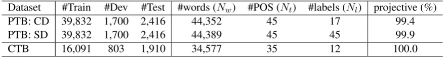
Table 3: Data Statistics. “Projective” is the percentage of projective trees on the training set.

and Nugues, 2007) using the LTH Constituent-to-Dependency Conversion Tool3_{and Stanford Basic}

Dependencies (SD) (de Marneffe et al., 2006) us-ing the Stanford parser v3.3.0.4 _{The POS tags are}

assigned using Stanford POS tagger (Toutanova et al., 2003) with ten-way jackknifing of the training data (accuracy≈97.3%).

For Chinese, we adopt the same split ofCTB5

as described in (Zhang and Clark, 2008). Depen-dencies are converted using the Penn2Malt tool5

with the head-finding rules of (Zhang and Clark, 2008). And following (Zhang and Clark, 2008; Zhang and Nivre, 2011), we use gold segmenta-tion and POS tags for the input.

Table 3 gives statistics of the three datasets.6 _In

particular, over 99% of the trees are projective in all datasets.

4.2 Results

The following hyper-parameters are used in all ex-periments: embedding sized = 50, hidden layer sizeh= 200, regularization parameterλ= 10−8_,

initial learning rate of Adagradα= 0.01.

To situate the performance of our parser, we first make a comparison with our own implementa-tion of greedy arc-eager and arc-standard parsers. These parsers are trained with structured averaged perceptron using the “early-update” strategy. The feature templates of (Zhang and Nivre, 2011) are used for the arc-eager system, and they are also adapted to the arc-standard system.7

Furthermore, we also compare our parser with two popular, off-the-shelf parsers: Malt-Parser — a greedy transition-based dependency parser (Nivre et al., 2006),8 _{and MSTParser —}

3_{http://nlp.cs.lth.se/software/treebank converter/} 4_{http://nlp.stanford.edu/software/lex-parser.shtml} 5_{http://stp.lingfil.uu.se/ nivre/research/Penn2Malt.html} 6_{Pennconverter and Stanford dependencies generate} slightly different tokenization, e.g., Pennconverter splits the tokenWCRS\/Boston NNPinto three tokensWCRS NNP /

CC Boston NNP.

7_{Since arc-standard is bottom-up, we remove all features} using the head of stack elements, and also add the right child features of the first stack element.

8_{http://www.maltparser.org/}

a first-order graph-based parser (McDonald and Pereira, 2006).9 _{In this comparison, for}

Malt-Parser, we selectstackproj(arc-standard) and

nivreeager(arc-eager) as parsing algorithms, and liblinear (Fan et al., 2008) for optimization.10

For MSTParser, we use default options.

On all datasets, we report unlabeled attach-ment scores (UAS) and labeled attachattach-ment scores (LAS) and punctuation is excluded in all evalua-tion metrics.11 _{Our parser and the baseline}

arc-standard and arc-eager parsers are all implemented in Java. The parsing speeds are measured on an Intel Core i7 2.7GHz CPU with 16GB RAM and the runtime does not include pre-computation or parameter loading time.

Table 4, Table 5 and Table 6 show the com-parison of accuracy and parsing speed on PTB (CoNLL dependencies), PTB (Stanford dependen-cies) and CTB respectively.

Parser _{UAS LAS UAS LAS (sent/s)}Dev Test Speed standard 89.9 88.7 89.7 88.3 51 eager 90.3 89.2 89.9 88.6 63 Malt:sp 90.0 88.8 89.9 88.5 560 Malt:eager 90.1 88.9 90.1 88.7 535 MSTParser 92.1 90.8 92.0 90.5 12 Our parser 92.2 91.0 92.0 90.7 1013 Table 4: Accuracy and parsing speed on PTB + CoNLL dependencies.

Clearly, our parser is superior in terms of both accuracy and speed. Comparing with the base-lines of arc-eager and arc-standard parsers, our parser achieves around 2% improvement in UAS and LAS on all datasets, while running about 20 times faster.

It is worth noting that the efficiency of our

9_{http://www.seas.upenn.edu/ strctlrn/MSTParser/} MSTParser.html

10_{We do not compare with libsvm optimization, which is} known to be sightly more accurate, but orders of magnitude slower (Kong and Smith, 2014).

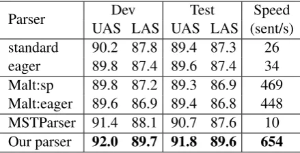
Parser _{UAS LAS UAS LAS (sent/s)}Dev Test Speed standard 90.2 87.8 89.4 87.3 26 eager 89.8 87.4 89.6 87.4 34 Malt:sp 89.8 87.2 89.3 86.9 469 Malt:eager 89.6 86.9 89.4 86.8 448 MSTParser 91.4 88.1 90.7 87.6 10 Our parser 92.0 89.7 91.8 89.6 654 Table 5: Accuracy and parsing speed on PTB + Stanford dependencies.

Parser _{UAS LAS UAS LAS (sent/s)}Dev Test Speed standard 82.4 80.9 82.7 81.2 72 eager 81.1 79.7 80.3 78.7 80 Malt:sp 82.4 80.5 82.4 80.6 420 Malt:eager 81.2 79.3 80.2 78.4 393 MSTParser 84.0 82.1 83.0 81.2 6 Our parser 84.0 82.4 83.9 82.4 936

Table 6: Accuracy and parsing speed on CTB.

parser even surpasses MaltParser using liblinear, which is known to be highly optimized, while our parser achieves much better accuracy.

Also, despite the fact that the graph-based MST-Parser achieves a similar result to ours on PTB (CoNLL dependencies), our parser is nearly 100 times faster. In particular, our transition-based parser has a great advantage in LAS, especially for the fine-grained label set of Stanford depen-dencies.

4.3 Effects of Parser Components

Herein, we examine components that account for the performance of our parser.

Cube activation function

We compare our cube activation function (x3₎

with two widely used non-linear functions:tanh

(ex_−e−x

ex_+e−x), sigmoid (₁₊1_e−x), and also the

identity function (x), as shown in Figure 4 (left).

In short,cubeoutperforms all other activation functions significantly andidentityworks the worst. Concretely, cube can achieve 0.8% ∼ 1.2%improvement in UAS overtanhand other functions, thus verifying the effectiveness of the cube activation function empirically.

Initialization of pre-trained word embeddings We further analyze the influence of using pre-trained word embeddings for initialization. Fig-ure 4 (middle) shows that using pre-trained word embeddings can obtain around 0.7% improve-ment on PTB and 1.7% improvement on CTB, compared with using random initialization within

(−0.01,0.01). On the one hand, the pre-trained word embeddings of Chinese appear more use-ful than those of English; on the other hand, our model is still able to achieve comparable accuracy without the help of pre-trained word embeddings.

POS tag and arc label embeddings

As shown in Figure 4 (right), POS embeddings yield around 1.7% improvement on PTB and nearly 10% improvement on CTB and the label embeddings yield a much smaller 0.3% and 1.4% improvement respectively.

However, we can obtain little gain from la-bel embeddings when the POS embeddings are present. This may be because the POS tags of two tokens already capture most of the label informa-tion between them.

4.4 Model Analysis

Last but not least, we will examine the parame-ters we have learned, and hope to investigate what these dense features capture. We use the weights learned from the English Penn Treebank using Stanford dependencies for analysis.

What doEt_,El_capture?

We first introduced Et _{and E}l _{as the dense} rep-resentations of all POS tags and arc labels, and we wonder whether these embeddings could carry some semantic information.

Figure 5 presents t-SNE visualizations (van der Maaten and Hinton, 2008) of these embeddings. It clearly shows that these embeddings effectively exhibit the similarities between POS tags or arc labels. For instance, the three adjective POS tags

JJ,JJR, JJS have very close embeddings, and also the three labels representing clausal comple-ments acomp, ccomp, xcomp are grouped to-gether.

What doWw

1 ,W1t,W1lcapture?

Knowing thatEt_andEl_{(as well as the word} em-beddings Ew_{) can capture semantic information} very well, next we hope to investigate what each feature in the hidden layer has really learned.

Since we currently only haveh = 200learned dense features, we wonder if it is sufficient to learn the word conjunctions as sparse indicator features, or even more. We examine the weights

Ww

1 (k,·) ∈ Rd·nw,W1t(k,·) ∈ Rd·nt,W1l(k,·)∈

Rd·nlfor each hidden unitk, and reshape them to d×nt, d×nw, d×nl matrices, such that the weights of each column corresponds to the embed-dings of one specific element (e.g.,s1.t).

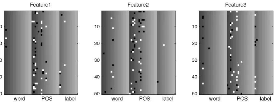
We pick the weights with absolute value>0.2, and visualize them for each feature. Figure 6 gives the visualization of three sampled features, and it exhibits many interesting phenomena:

• Different features have varied distributions of the weights. However, most of the discrim-inative weights come from Wt

1 (the middle

zone in Figure 6), and this further justifies the importance of POS tags in dependency pars-ing.

• We carefully examine many of theh = 200

features, and find that they actually encode very different views of information. For the three sampled features in Figure 6, the largest weights are dominated by:

– Feature 1:s1.t, s2.t, lc(s1).t.

– Feautre 2:rc(s1).t, s1.t, b1.t.

– Feature 3:s1.t, s1.w, lc(s1).t, lc(s1).l.

These features all seem very plausible, as ob-served in the experiments on indicator feature systems. Thus our model is able to automati-cally identify the most useful information for predictions, instead of hand-crafting them as indicator features.

• More importantly, we can extract features re-garding the conjunctions of more than3 ele-ments easily, and also those not presented in the indicator feature systems. For example, the 3rd feature above captures the conjunc-tion of words and POS tags ofs1, the tag of

its leftmost child, and also the label between them, while this information is not encoded in the original feature templates of (Zhang and Nivre, 2011).

5 Related Work

There have been several lines of earlier work in us-ing neural networks for parsus-ing which have points of overlap but also major differences from our work here. One big difference is that much early work uses localist one-hot word representations rather than the distributed representations of mod-ern work. (Mayberry III and Miikkulainen, 1999) explored a shift reduce constituency parser with one-hot word representations and did subsequent parsing work in (Mayberry III and Miikkulainen, 2005).

(Henderson, 2004) was the first to attempt to use neural networks in a broad-coverage Penn Tree-bank parser, using a simple synchrony network to predict parse decisions in a constituency parser. More recently, (Titov and Henderson, 2007) ap-plied Incremental Sigmoid Belief Networks to constituency parsing and then (Garg and Hender-son, 2011) extended this work to transition-based dependency parsers using a Temporal Restricted Boltzman Machine. These are very different neu-ral network architectures, and are much less scal-able and in practice a restricted vocabulary was used to make the architecture practical.

There have been a number of recent uses of deep learning for constituency parsing (Collobert, 2011; Socher et al., 2013). (Socher et al., 2014) has also built models over dependency representa-tions but this work has not attempted to learn neu-ral networks for dependency parsing.

Most recently, (Stenetorp, 2013) attempted to build recursive neural networks for transition-based dependency parsing, however the empirical performance of his model is still unsatisfactory.

6 Conclusion

We have presented a novel dependency parser us-ing neural networks. Experimental evaluations show that our parser outperforms other greedy parsers using sparse indicator features in both ac-curacy and speed. This is achieved by represent-ing all words, POS tags and arc labels as dense vectors, and modeling their interactions through a novel cube activation function. Our model only relies on dense features, and is able to automat-ically learn the most useful feature conjunctions for making predictions.

PTB:CD PTB:SD CTB 80 85 90 U AS score

cube tanh sigmoid identity

PTB:CD PTB:SD CTB

80 85 90 U AS score pre-trained random

PTB:CD PTB:SD CTB

70 75 80 85 90 95 U AS score

word+POS+label word+POS word+label word

Figure 4: Effects of different parser components. Left: comparison of different activation functions. Middle: comparison of pre-trained word vectors and random initialization. Right: effects of POS and label embeddings.

−600 −400 −200 0 200 400 600

−800 −600 −400 −200 0 200 400 600 −ROOT− IN DT NNP CD NN ‘‘ ’’ POS ( VBN NNS VBP , CC ) VBD RB TO . VBZ NNPS PRP PRP$ VB JJ MD VBG RBR : WP WDT JJR PDT RBS WRB JJS $ RP FW EX SYM # LS UH WP$ misc noun punctuation verb adverb adjective

−600 −400 −200 0 200 400 600 800 −1000 −800 −600 −400 −200 0 200 400 600 800 neg acomp det predet root infmod cop quantmod nn conj nsubj aux npadvmod csubj mwe possessive expl auxpass csubjpass advcl pcomp discourse dep partmod poss advmod appos prt number mark dobj parataxis prep ccomp num punct rcmod xcomp preconj pobj nsubjpass iobj amod cc tmod misc clausal complement noun pre−modifier verbal auxiliaries subject preposition complement noun post−modifier

Figure 5: t-SNE visualization of POS and label embeddings.

Figure 6: Three sampled features. In each feature, each row denotes a dimension of embeddings and each column denotes a chosen element, e.g., s1.t orlc(s1).w, and the parameters are divided into 3

zones, corresponding toWw

1 (k,:)(left),W1t(k,:)(middle) andW1l(k,:)(right). White and black dots

there is still room for improvement in our architec-ture, such as better capturing word conjunctions, or adding richer features (e.g., distance, valency).

Acknowledgments

Stanford University gratefully acknowledges the support of the Defense Advanced Research Projects Agency (DARPA) Deep Exploration and Filtering of Text (DEFT) Program under Air Force Research Laboratory (AFRL) contract no. FA8750-13-2-0040 and the Defense Threat duction Agency (DTRA) under Air Force Re-search Laboratory (AFRL) contract no. FA8650-10-C-7020. Any opinions, findings, and conclu-sion or recommendations expressed in this mate-rial are those of the authors and do not necessarily reflect the view of the DARPA, AFRL, or the US government.

References

Bernd Bohnet. 2010. Very high accuracy and fast de-pendency parsing is not a contradiction. InColing.

Ronan Collobert, Jason Weston, L´eon Bottou, Michael Karlen, Koray Kavukcuoglu, and Pavel Kuksa. 2011. Natural language processing (almost) from scratch. Journal of Machine Learning Research. Ronan Collobert. 2011. Deep learning for efficient

discriminative parsing. InAISTATS.

Marie-Catherine de Marneffe, Bill MacCartney, and Christopher D. Manning. 2006. Generating typed dependency parses from phrase structure parses. In LREC.

Jacob Devlin, Rabih Zbib, Zhongqiang Huang, Thomas Lamar, Richard Schwartz, and John Makhoul. 2014. Fast and robust neural network joint models for sta-tistical machine translation. InACL.

John Duchi, Elad Hazan, and Yoram Singer. 2011. Adaptive subgradient methods for online learning and stochastic optimization. The Journal of Ma-chine Learning Research.

Rong-En Fan, Kai-Wei Chang, Cho-Jui Hsieh, Xiang-Rui Wang, and Chih-Jen Lin. 2008. Liblinear: A library for large linear classification. The Journal of Machine Learning Research.

Nikhil Garg and James Henderson. 2011. Temporal restricted boltzmann machines for dependency pars-ing. InACL-HLT.

He He, Hal Daum´e III, and Jason Eisner. 2013. Dy-namic feature selection for dependency parsing. In EMNLP.

James Henderson. 2004. Discriminative training of a neural network statistical parser. InACL.

Geoffrey E. Hinton, Nitish Srivastava, Alex Krizhevsky, Ilya Sutskever, and Ruslan Salakhut-dinov. 2012. Improving neural networks by preventing co-adaptation of feature detectors. CoRR, abs/1207.0580.

Liang Huang, Wenbin Jiang, and Qun Liu. 2009. Bilingually-constrained (monolingual) shift-reduce parsing. InEMNLP.

Richard Johansson and Pierre Nugues. 2007. Ex-tended constituent-to-dependency conversion for en-glish. InProceedings of NODALIDA, Tartu, Estonia. Lingpeng Kong and Noah A. Smith. 2014. An em-pirical comparison of parsing methods for Stanford dependencies. CoRR, abs/1404.4314.

Terry Koo, Xavier Carreras, and Michael Collins. 2008. Simple semi-supervised dependency parsing. InACL.

Sandra K¨ubler, Ryan McDonald, and Joakim Nivre. 2009. Dependency Parsing. Synthesis Lectures on Human Language Technologies. Morgan & Clay-pool.

Marshall R. Mayberry III and Risto Miikkulainen. 1999. Sardsrn: A neural network shift-reduce parser. InIJCAI.

Marshall R. Mayberry III and Risto Miikkulainen. 2005. Broad-coverage parsing with neural net-works. Neural Processing Letters.

Ryan McDonald and Fernando Pereira. 2006. Online learning of approximate dependency parsing algo-rithms. InEACL.

Tomas Mikolov, Ilya Sutskever, Kai Chen, Greg S Cor-rado, and Jeff Dean. 2013. Distributed representa-tions of words and phrases and their compositional-ity. InNIPS.

Joakim Nivre, Johan Hall, and Jens Nilsson. 2006. Maltparser: A data-driven parser-generator for de-pendency parsing. InLREC.

Richard Socher, John Bauer, Christopher D Manning, and Andrew Y Ng. 2013. Parsing with composi-tional vector grammars. InACL.

Richard Socher, Andrej Karpathy, Quoc V. Le, Christo-pher D. Manning, and Andrew Y. Ng. 2014. Grounded compositional semantics for finding and describing images with sentences. TACL.

Pontus Stenetorp. 2013. Transition-based dependency parsing using recursive neural networks. In NIPS Workshop on Deep Learning.

Kristina Toutanova, Dan Klein, Christopher D. Man-ning, and Yoram Singer. 2003. Feature-rich part-of-speech tagging with a cyclic dependency network. InNAACL.

Laurens van der Maaten and Geoffrey Hinton. 2008. Visualizing data using t-SNE. The Journal of Ma-chine Learning Research.

Yue Zhang and Stephen Clark. 2008. A tale of two parsers: Investigating and combining graph-based and transition-graph-based dependency parsing us-ing beam-search. InEMNLP.