Abstract— The main purpose of this paper is to present of how
to use heuristic approaches, especially genetic algorithms, to a scenario manipulation in two-stage stochastic programming. Algorithms developed for two-stage stochastic linear programs usually require a solution of large-scale linear and nonlinear programs because the deterministic reformulations of original programs are based on empirical or sampling discrete probability distributions, i.e. on so-called scenario sets. As these sets are often huge, the reformulated programs must be simplified, and therefore, the scenario set reduction techniques are required. Hence, randomly selected reduced scenario sets are often employed. Related confidence intervals for the optimal objective function values have been derived and are often presented as tight enough. However, there is also demand for goal-oriented scenario manipulations. Traditional deterministic techniques are limited by the size of scenario set. Therefore, this paper introduces a possibility how to modify scenario sets by using heuristic algorithms. As an example, the search of absolute lower and upper bounds by using genetic algorithm is presented and further enhancements are discussed. The proposed technique is implemented in C++ and GAMS and then tested on real-data examples.
Index Terms— Stochastic programming, scenarios, worst case
analysis, heuristic and genetic algorithms.
I. BASIC CONCEPTS OF STOCHASTIC PROGRAMMING We denote a mathematical program as
( )
{
f ∈C}
∈argmin x x
? . Then, we naturally obtain an
underlying program ?∈argmin
{
f( )
x,ξ x∈C( )
ξ}
, as we replaced several original constant parameters by random elements. There is ξ , a random vector defined on the probability space(
Ξ,Σ,Ρ)
, and :IRn×Ξ→IRf , is a
measurable function for each decision x∈IRn that must
belong to the feasible set C. To be able to solve optimization problem correctly, the deterministic reformulation must be
Manuscript received July 22 2007. This work has been supported by the Czech Ministry of Education in the frame of MSM 0021630529 Intelligent Systems in Automation and by the GA CR project: 103/05/0292 and the CQR
research center of the Czech Republic.
J. Roupec is with the Institute of Automation and Computer Science, Faculty of Mechanical Engineering, Brno University of Technology, Technicka 2, 616 69 Brno, Czech Republic (phone: +420 54114 3346; e-mail: [email protected]).
P. Popela is with the Institute of Mathematics, Faculty of Mechanical Engineering, Brno University of Technology, Technicka 2, 616 69 Brno, Czech Republic (e-mail: [email protected]).
further specified. Usually, we cannot wait for observation ξs,
and we must decide here-and-now. In this case, we have to utilize suitable HN-reformulation and we have chosen the most typical one:
( )
( )
{
, a.s.}
min arg
? ξ xξ x ξ
x
C f
E ∈
∈ , (1)
where E denotes expectation functional and abbreviation a.s. means almost surely. However, there are also different approaches to random parameter modeling, see, e.g., [6] for details.
It is difficult to solve the stochastic program (1) in the case when the random vector has the continuous probability distribution. Then, the approximation techniques based on discretization are used, see [6]. So, we focus on a finite support case. For the discrete random vector ξ, instead of solution difficulty related to multidimensional integration to compute E, we have to deal with the computational complexity caused by the HN-reformulation size. Particularly, E is computed explicitly as we may denote
( )
ss P
p = ξ=ξ and write the expectation as a sum. Therefore, the SB-reformulation is a large nonlinear program:
( )
( )
⎭ ⎬ ⎫ ⎩
⎨ ⎧
∈ Σ
∈
Ξ ∈ Ξ
∈
s s
sf C
p
s
s xξ x ξ ξ
ξ
x I
, min
arg
? . (2)
The main problem is of how to choose suitable realizations
s
ξ called scenarios when only incomplete information about the probability distribution is available. The scenario-related techniques are discussed in the paper [3], an interesting approach is proposed in [5].
II. TEST EXAMPLES
A scenario-based (SB), two-stage stochastic linear program, modeling a principal part of a melt control process in a suitable furnace (cupola, induced, or electric-arc) is chosen as an example for further computations because it allows to use real world data and can be easily modified, see [13] for details.
( )
( )
{
}
S sQ
Q p
s s
s
s s
s s
S s
s s x
s
, , 1 , 0 , ,
, min
;
0 ;
min arg ?
2 2 1 1
2 2 1 1 T
1 T
K
= ≥ ≥
+
≥ + =
⎭ ⎬ ⎫ ⎩
⎨ ⎧
≥ +
∈
∑
=
y x u y A x A T
l y A x A T y q
ξ
x
x
ξ
x x
c
y (3)
where x is a tonnage of n1 charge materials and ys
Scenario Generation And Analysis by Heuristic
Algorithms
represents a tonnage of n2 alloying materials. Symbols l2 and 2
u describe a minimum and maximum tonnage of m considered elements after alloying. Then, A1 is a matrix containing the known proportions aij of ith element in jth charge material and A2 is a matrix containing information
about alloying materials.
{
ξ1, ,ξs}
K
=
Ξ is a finite support of distribution ξ that is composed of scenarios ξs (or shortly
s),
and
(
)
s Ss P
ps = ξ=ξs =1, =1,K, . The random utilization of elements in the charge melt is therefore defined by s
1
T . The alloying utilization is described by the unit matrix I that stays in front of A2. The overall expected cost of repeated similar melts is minimized, therefore, c and q are vectors representing costs per ton for input materials. The discussed melt control model development is described in [10]-[14]. The developed techniques are related to material engineering approaches in [7] and [8].
Utilization matrix s
1
Τ has a diagonal form and we denote
33 3 22 2 11
1s =ts,τs =ts ,t =t
τ , and t4 =t44. Firstly, we assumed only two random diagonal elements to simplify the results analysis. As the next step, we have assumed all diagonal elements random. The largest problem solved with real data dealt with 16 random elements of the diagonal of utilization matrix. We assign remaining utilization t3 =0.7 and t4 =1.
We denote τ=
(
τ1,τ2)
T and we assume that(
0.734;0.866)
1≈U
τ and τ2≈U
(
0.902;0.998)
are independent random variables with continuous discrete probability distribution (for next computations:(
0.672;0.733)
3≈Uτ and τ4≈U
(
0.972;1.000)
). Then, τs are realizations of τ. Input data in Table I is significantly modified in comparison with [17] and [19] as we generalized the previous simple recourse case, see Table I.III. SAMPLING TECHNIQUES
We want to compute the optimal HN-solution xHNmin and
related objective function value HN min
z . One possible way is to approximate it and reduce a program size with random sampling. We denote a random sample from ξ as
[].
(
ξ[ ]1, ,ξ[ ]ν)
Tξ = K . There are ξ[ ]s random variables identically distributed as ξ and they are stochastically independent. The realization of this random sample is usually denoted as ξs[]. =
(
ξ[ ]s1,K,ξs[ ]ν)
T. We often simplify our notation as follows: ξ[]s.(
ξs1, ,ξsν)
TK
= . For computational purposes, we may easily replace Eξ
{
f( )
x,ξ}
(and hence Eξ{
Q( )
x,ξ}
for two-stage programs) by the realization of a sample mean( )
∑
=ν
ν 1 ,
1
s s
f xξ (and
∑
ν=( )
ν 1 ,
1
s s
Qxξ for two-stage programs):
(
)
( )
⎭⎬⎫ ⎩ ⎨ ⎧ ∈ = =∑
∑
= = ν ν ν ν ν ν 1 1 ´ min min , 1 min ; 1 s s s s C f fz x ξ xξ x
x (4)
Randomly generated observations of ξ may then serve to compute the estimate of the objective (and recourse) function. Therefore, scenarios are selected by random procedure. Then, the scenarios ξs are used to build a scenario tree, and this
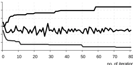
reduced program is solved instead of the original one. However, its blindfold and exaggerated use can lead to misleading results. So, in addition, Monte Carlo techniques may be necessary to obtain an estimate of how good is such a simplification. Then, repeated computations inform us about the result stability and sensitivity, see the piece-wise linear line in the middle of Fig. 1. The reduction of the objective function estimate variance is also illustrated.
Morton, Mak, and Wood prove in [9] the following inequalities:
{ } { }
min E min1 zminHN z E{
f( )
x;ξ}
Eξ ςν ≤ ξ ςν+ ≤ ≤ = ξ , (5)
where x is any feasible solution from C. They assume that a random sample from ξ denoted as ξ[]. =
(
ξ[ ]1,K,ξ[ ]νu)
T is available and the ς denotes a random optimal objective function value depending on the random sample. They have νl random samples, each having size ν , therefore[ ].
(
[ ]1, , [ ])
T: , ,
14 νl i i iν
i= K ξ = ξ Kξ
∀ . They use inequalities (5)
and the central limit theorem to derive the following bounds:
[ ] ( )
(
( )
[ ] [ ])
( )
[ ] ⎭⎬−( )
≤ ⎫ ⎩ ⎨ ⎧ ∈ ⎜ ⎜ ⎝ ⎛ − = =∑
∑
l l l s i is i i l s t C f P l i ν ν ν ν α νν 1 2
1 . .
1 a.s. ; 1 min 1 . ξ x ξ ξ x ξ x
{ }
≤ ≤{
( )
}
≤≤ ξς HN ξ x;ξ
min
min z E f
E ν (6)
[ ]
(
)
( )
αν ν ν α ν − ≈ ⎟ ⎟ ⎠ ⎞ + ≤ − = +
∑
; 11 1 2
1 l l l s s u s t
f xξ .
The symbol t1−α 2 denotes the 1−α 2 quantile of N
( )
0;1 distribution. Symbols sl( )
νl and su( )
νu denote usualestimates of standard deviations varςνmin and varf
( )
x;ξ .Hence, we may set α, then substitute observations []s
.
ξ and
[]
s i.
ξ in the formula (6), and we obtain reliable bounds. IV. EXTREME SCENARIO SETS
We may see that for our melt control example, a resulted sequence of optimum objective values for different samples is on Figure 1 (the line in the middle). The aforementioned bounds in this case are also very promising. However, still one question remains. Are they so good because of small influence of randomness or only ‘dangerous’ scenarios are not participating in our samples?
follows (see [12] and [14]):
( )
( )
⎪⎭ ⎪ ⎬ ⎫ ⎪⎩
⎪ ⎨ ⎧
∈
∑
∈ =⊂ S s
s s
n S
S s
C f
Sξ
Ξ x;ξ x
I
ξ1 min min
; (7)
( )
( )
⎪⎭ ⎪ ⎬ ⎫ ⎪⎩
⎪ ⎨ ⎧
∈
∑
∈ =⊂ S s
s s
n S
S s
C f
Sξ
Ξ x;ξ x
I
ξ1 min max
; (8)
Because the objective function convexity with respect to ξ is not guaranteed in general case, this problem might be quite difficult to solve. Because of the problem size, it is also impossible to consider all scenarios as Rosa and Takriti in [15] and try to exclude certain scenarios computing the whole optimization program that sets their probabilities to zero.
V. ALGORITHMS
The basic idea of a genetic algorithm (GA) is quite simple. GA works not only with one solution in time but with the whole population of solutions. The population contains many (ordinary several hundreds) individuals – bit strings representing solutions. The mechanism of GA involves only elementary operations like strings copying, partially bit swapping or bit value changing. GA starts with a population of strings and thereafter generates successive populations using
the following three basic operations: reproduction, crossover, and mutation. Reproduction is the process by which individual strings are copied according to an objective function value (fitness). Copying of strings according to their fitness value means that strings with a higher value have a higher probability of contributing one or more offspring to next generation. This is an artificial version of natural selection. Mutation is an occasional (with a small probability) random alteration of the string position value. Mutation is needed since, in spite of reproduction and crossover effectively searching and recombining the existing representations, they occasionally become overzealous and lose some potentially useful genetic material. The mutation operator prevents such an irrecoverable loss. The recombination mechanism allows mixing of parental information while passing it to their descendants, and mutation introduces innovation into the population. When you submit your final version, after your paper has been accepted, prepare it in two-column format, including figures and tables.
In spite of simple principles, the design of GA for successful practical using is surprisingly complicated. GA has many parameters that depend on the problem to be solved. In the first, it is the size of population. Larger populations usually decrease the number of iterations needed, but dramatically increase the computing time for each of iteration. The factors increasing
Elements Solution
St. Alloys C Mn Si Cr Bounds Prices EV
t j i:A1T,AT2 b c, q xEVmin xLOmin−UP
1 Iron 5 0.947 3.124 0 ∞ 60.0 0.73713 0.67858
1 Spinput 0 4.737 21.429 10 ∞ 129.0 0.03000 0.03000
1 FeSi-1 0 0 64.286 0 ∞ 130.0 0.00000 0.00000
1 FeSi-2 0 0 60.000 0 ∞ 122.0 0.01103 0.01437
1 Alloy-1 0 63.158 25.714 0 ∞ 200.0 0.00712 0.00664
1 Alloy-2 0 9.474 42.857 20 ∞ 260.0 0.00000 0.00000
1 Alloy-3 0 34.737 35.714 8 ∞ 238.0 0.00000 0.00000
1 SiC 18.75 0 42.857 0 0.01 160.0 0.00000 0.00000
1 Steel-1 0.5 0.947 0 0 0.1000 42.0 0.10000 0.10000
1 Steel-2 0.125 0.316 0 0 0.1000 40.0 0.01472 0.07041
1 Steel-3 0.125 0.316 0 0 0.1000 39.0 0.10000 0.10000
2 A-C 100 0 0 0 ∞ 800 0.007 0.00457
2 A-Mn 2 70 10 4 ∞ 1500 0.005 0.00130
2 A-Si 1 0 60 0 ∞ 1900 0.001 0.0005
2 A-Cr 1 6 1 40 ∞ 4000 0.001 0.0007
2
I
3 1.35 2.7 0.3Mix 3.75 1.421 3.857 0.3
( )
E
ξ
T
1 0.8 0.95 0.7 1melt result 3 1.35 2.7 0.3
z
min 67.5562
u
3.5 1.65 3.0 0.45E
{ }
z
min 83.176 69.5702demands on the size of population are the complexity of the problem being solved and the length of the individuals. Every individual contains one or more chromosomes containing value of potential solution. Chromosomes consist of genes. The gene in our version of GA is a structure representing one bit of solution value. It is usually advantageous to use some redundancy in genes and so the physical length of our genes is greater than one bit. This type of redundancy was introduced by Ryan [20].
To prevent degeneration and the deadlock in local extreme the limited lifetime of individual can be used. Limited lifetime is realized by the “death” operator [21], which represents something like continual restart of GA. This operator enables decreasing of population size as well as increasing the speed of convergence. It is necessary to store the best solution obtained separately – the corresponding individual need not to be always present in the population because of the limited lifetime.
Many GAs are implemented on a population consisting of haploid individuals (each individual contains one chromosome). However, in nature, many living organisms have more than one chromosome and there are mechanisms used to determine dominant genes. Sexual recombination generates an endless variety of genotype combination that increases the evolutionary potential of the population. Because it increases the variation among the offspring produced by an individual, it improves the change that some of them will be successful in varying and often-unpredictable environments they will encounter. Using diploid or “multiploid” individuals can often decrease demands on the population size. However the use of multiploid GA with sexual reproduction brings some complications, the advantage of multiploidity can be often substitute by the “death” operator and redundant genes coding.
New individuals are created by operation called crossover. In the simplest case crossover means swapping of two parts of two chromosomes split in randomly selected point (so called one point crossover). In GA we use the uniform crossover on the bit level is used.
The strategy of selection individuals for crossover is very important. It strongly determines the behavior of GA. For grammatical evolution the ranking selection with elite brings satisfactory results.
Genetic algorithms commonly use heuristic and stochastic approaches. From the theoretical viewpoint, the convergence of
heuristic algorithms is not guaranteed for the most of application cases. That is why the definition of the stopping rule of the GA brings a new problem. It can be shown [22], that while using a proper version of GA the typical number of iterations can be determine.
GAs we use have the following scheme:
1. Generation of the initial population: At the beginning the whole population is generated randomly, the members are sorted by the fitness (in descendent order). 2. Mutation: The mutation is applied to each gene with the
same probability, all GAs we used use pmut = 0.05. The
mutation of the gene means the inversion of one randomly selected bit in the gene.
3. Death: Classical GA uses two main operations – crossover and mutation (the other operation should be migration). In GA described in this paper, we use the third operation – death. Every individual has the additional information – age. A simple counter that is incremented in each of GA iteration represents the age. If the age of any member reaches the preset lifetime limit LT, this member "dies" and is immediately replaced by a new randomly generated member. The age is not mutated nor crossed over. The age of new individuals (incl. individuals created by crossover) is set to zero. Lifetime limit in our application is set to 5. 4. Sorting by the fitness.
5. Crossover: Uniform crossover is used for all genes (each bit of the offspring gene is selected separately from corresponding bits of both parents genes). 6. When a stopping rule is not satisfied, go to step 2. In crossover, we do not replace all members of the population. The crossover generates the number of individuals corresponding to the quarter of the population only. Created individuals are sorted into the corresponding places in the population according to their fitness in such a way that the size of the population remains the same. Newly created individuals of low fitness do not have to be involved in the population.
So, we assume that components of discrete random vector ξ are independent random variables with finite supports. We suggest a usual algorithm for general case of finite marginal supports Ξi. Evolutionary and genetic algorithms were already used in stochastic programming by Berland in [1] and a group of authors [18]. The changing set of scenarios S (7) is considered as a population. For each member of this population, the objective function value is computed by running an external program in GAMS [2] that allows various modifications of the model (3). Therefore, for given S and the optimal solution xmin (similarly for xmax and (8)) of (7), we
calculate
{
f(
x ;ξs)
min . Then the population is ordered by
fitness values, and usual operations as reproduction, crossover, and mutation are realized.
[image:4.595.46.281.87.201.2]Main search algorithm. At the end of this section, we describe the basic loop of main algorithm that searches extreme scenario sets:
Fig. 1 - Development of various objective function values computed by GA
0 0,2 0,4 0,6 0,8 1 1,2
0 10 20 30 40 50 60 70 80
1. During initialization, a main program controlling the whole computational process is started. It reads optimization engine name (GAMS [2] in our example), main source filename, included filename with scenarios, filename for melt control results, filename for GA input, number of scenarios, dimension, and distribution of τ. 2. The main program calls the optimization engine, and it
solves the SB-program. Input data for GA is generated; it includes fitness values related to scenarios.
3. Then, the GA starts and generates a new set of scenarios. 4. When a stopping rule is not satisfied, continue by step 2.
VI. RESULTS AND FURTHER RESEARCH
We have applied the aforementioned main algorithm together with GAMS source for (3) and discussed GA. As a result we obtained a sequence of randomly selected scenario sets together with sequences of searched pairs of extreme sets. Figure 1 presents the development of related objective function values (see [7] and [8]) for the case of diagonal with 4 random elements and implemented genetic algorithm. It is clearly visible, how the modified GA quickly searches for the both bounds. The aforementioned confidence intervals are significantly tighter even in the case of increased confidence level, hence may be interpreted as too optimistic for the situation when the worst case analysis is the goal. The algorithm proved the significant improvement in comparison with [19].
Further research will be focused on postoptimality analysis realized with respect to the original set of scenarios. Mainly, the cases where the incomplete recourse [6] appears to be very important, will be studied. We assume that the deeper understanding of the whole algorithm behaviour will lead to the used GA improvement.
The used test problems are derived from the underlying linear programs, therefore, the proposed technique will be applied to nonlinear programming engineering applications, e.g., in reliable structural design.
REFERENCES
[1] N. J. Berland, Stochastic Optimization and Parallel Processing. PhD
thesis, University of Bergen, 1993.
[2] A. Brooke, D. Kendrick, and A. Meeraus. Release 2.25 GAMS A User's Guide. The Scientific Press. Boyd & Fraser Publishing Company, 2nd edition, 1992.
[3] J. Dupačová, G. Consigli, and S. W. Wallace, “Scenarios for multistage stochastic programs,” Annals of Operations Research, 100: 25–53, 2000. [4] W. H. Evers, “A new model for stochastic linear programming,”
Management Science, 13:680–693, 1967.
[5] K. Hoyland and S. W. Wallace, Generating scenario trees for multi stage problems. Technical Report 4/97, Department of Industrial Economics and Technology Management, Norwegian University of Science and Technology, Trondheim, 1996.
[6] P. Kall and S. W. Wallace, Stochastic Programming. John Wiley and Sons, Chichester, 1994.
[7] Z. Karpíšek. “Heterogenity characteristics of cast iron alloying elements,”
Folia Fac. Sci. Nat. Univ. Masarykianae, Mathematica, 7:31–36, 1998.
[8] F. Kavička, K. Stránský, J. Stětina, V. Dobrovská, J. Dobrovská, and B. Velička. “Contribution to optimization of continuous casting of steel,”
Acta Metallurgica Slovaca, 5:367–370, 1999.
[9] W. K. Mak, D. P. Morton, and R. K. Wood, “Monte Carlo bounding techniques for deterministic solution quality in stochastic programs,”.
Operations Research Letters, 24:47–56, 1999.
[10] P. Popela, “A multistage blending problem with an expert estimate of parameters” (in Czech), in Proceedings of 3μ Conference on Modern Mathematical Methods, Ostrava, Czech Republic, 1994, pp 101–105.
[11] P. Popela and R. Setnička, Analysis of steel production (in Czech). Technical report, ŽĎAS, Žďár nad Sázavou, Czech Republic, 1995. [12] P. Popela, “Advanced scenario tuning in stochastic programming,” in
Proceedings of Czech-Slovak-Japan Workshop, Bratislava, Slovakia,
1998, pp. 307–310.
[13] P. Popela, “Application of stochastic programming in foundry,” Folia Fac. Sci. Nat. Univ. Masarykianae Brunensis, Mathematica, 7:117–139,
1998.
[14] P. Popela, An Object-Oriented Approach to Multistage Stochastic Programming: Models and Algorithms, PhD thesis, Charles University, Prague, 1998.
[15] C. H. Rosa and S. Takriti, A minimax formulation for stochastic programs using scenario aggregation, Technical report, SABRE Dec. Technol. and IBM T. J. Watson Center, July 17 1997.
[16] Y. Yoshitomi, T. Takeba, S. Tomita, and H. Ikenoue, “Genetic algorithm approach for solving stochastic programming problems,” in Proceedings of International Conference on Stochastic Programming, Vancouver, Canada, 1998.
[17] J. Zeman, Optimization models in metallurgy (in Czech), Master thesis,
Dept. of Math., FME Brno University of Technology, Brno, Czech Republic, 1998.
[18] J. Sklenar, “Simulation of Queuing Systems in QUESIM,” in Proceedings of the 2005 European Simulation and Modelling Conference ESM2005,
Riga, Latvia, 2005, pp. 35-37.
[19] P. Popela and J. Roupec, “GA-Based Scenario Set Modification in Two-Stage Melt Control Problems,” in Proceedings of the 5th International Conference MENDEL’99, Brno, Czech Republic, 1999,
pp.112–117.
[20] C. Ryan, “Shades. Polygenic Inheritance Scheme,” in Proceedings of the 3th International Conference on Soft Computing MENDEL ’97, Brno,
Czech Republic, 1997. pp. 140 – 147.
[21] J. Roupec, Design of Genetic Algorithm for Optimization of Fuzzy Controllers Parameters. (In Czech) PhD Thesis. Brno University of Technology, Brno, Czech Republic, 2001.