Extracting Morphophonology from Small Corpora

Proceedings of the 15th SIGMORPHON Workshop on Computational Research in Phonetics, Phonology, and Morphology, pages 167–175 167

Extracting morphophonology from small corpora

Marina Ermolaeva

University of Chicago / Chicago, IL, USA

[email protected]

Abstract

Probabilistic approaches have proven them-selves well in learning phonological struc-ture. In contrast, theoretical linguistics usu-ally works with deterministic generalizations. The goal of this paper is to explore possi-ble interactions between information-theoretic methods and deterministic linguistic knowl-edge and to examine some ways in which both can be used in tandem to extract phonological and morphophonological patterns from a small annotated dataset. Local and nonlocal pro-cesses in Mishar Tatar (Turkic/Kipchak) are examined as a case study.

1 Introduction

Morphophonology, or the interface between mor-phology and phonology, encompasses a wide range of phenomena. While this paper primar-ily focuses on learning phonological rules from a dataset, it is difficult to draw generalizations based only on surface strings, since the rules may be morphologically specific. The challenge goes be-yond learning which phonotactic sequences are al-lowed, also incorporating surface realizations of morphemes and rules governing their distribution. Large unannotated corpora are used by a large portion of the existing work on learning phono-logical patterns e.g. approaches to learning vowel harmony (Goldsmith and Riggle 2012;Szab´o and C¸ ¨oltekin 2013;Flinn 2014). However, in the case of rare languages, a large corpus may be unavail-able. On the other hand, small hand-annotated examples or texts are a natural output of linguis-tic fieldwork and readily available even for under-resourced and under-studied languages.

Interlinear glossed text is a format tradition-ally utilized in linguistic papers for presenting lan-guage data. It annotates each morpheme with a label, orgloss tag. When the amount of data is in-sufficient, the role of such linguistic knowledge in

making generalizations becomes more prominent; see (Wax 2014;Zamaraeva 2016) for approaches to extraction of morphological rules that take this path.

When it comes to morphophonology, agglutina-tive languages are of special interest. They tend to exhibit a variety of interacting processes which give rise to multiple surface realizations of most morphemes.1 A small dataset is very likely to con-tain only a subset of possible allomorphs – an ad-ditional challenge for the learning algorithm. As a case study, this paper focuses on Mishar dialect of Tatar language (Turkic/Kipchak). The data sample used here is a hand-glossed collection of texts elicited from native speakers in the course of fieldwork (MSU linguistic expedition 1999–2012) (3090 word tokens; 1740 types).

2 (Morpho)phonological processes

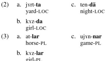
One common type of alternations stems from lo-cal processes, where the context is immediately adjacent to the segment undergoing the change. The same surface segment may arise from differ-ent processes. For example, the ablative suffix (1) has different realizations after voiceless con-sonants, nasals, and elsewhere. The locative mor-pheme (2) demonstrates only a two-way distinc-tion after voiceless consonants and elsewhere. The plural suffix (3) is also sensitive to a two-way dis-tinction, drawing a line between nasal consonants and other segments.

(1) a. kibet-t¨an shop-ABL

b. k7z-dan girl-ABL

c. ur7n-nan place-ABL

1_{For example, the idea of correlation between}

(2) a. j7rt-ta yard-LOC

b. k7z-da girl-LOC

c. ten-d¨a night-LOC

(3) a. at-lar horse-PL

b. k7z-lar girl-PL

c. uj7n-nar game-PL

While this data does hint at certain general phono-tactic patterns (e.g. a voiceless stop is never fol-lowed by an affix beginning with a voiced obstru-ent), the contexts cannot be inferred exclusively from surface strings; each morpheme has to be considered separately. Moreover, even the same set of alternants may be found in multiple pro-cesses. Consider the following voicing alterna-tion:

(4) a. matur-l7g-7 pretty-NOMIN-P3

b. jaxˇs7-l7k-ka good-NOMIN-DAT

(5) a. kal-gan stay-PFCT

b. ˇc7k-kan exit-PFCT

The difference between (4) and (5) lies in the di-rectionalityof the{g, k}alternation: the obstruent in the former is located at the left edge of the affix and assimilated to the preceding segment; in the latter it is sensitive to the voicing of the following segment.

Another prominent source of allomorphy is vowel harmony. This process is nonlocal in the sense that it only affects a subset of segments (in this case, the set of vowels); all other segments are transparent and do not interact with the rule in any way. Vowel harmony can be analyzed of in terms ofunderspecification(Archangeli 1988): vowels in affixes lack some feature specifications, and their surface realization is dependent on the closest fully specified vowel.

In Mishar Tatar, vowels are subject to fronting harmony controlled by the root; most affixes have front and back allomorphs.

[−BK,

−RND]

[−BK,

+RND]

[+BK,

−RND]

[+BK,

+RND] [+HI,−LO] i ¨u 7j u [−HI,−LO] e (¨o) 7 (o) [−HI,+LO] ¨a a

Table 1: Mishar Tatar vowels

(6) a. bala-lar-7b7z-ga child-PL-P1PL-DAT

b. t¨ar¨az-l¨ar-ebez-g¨a window-PL-P1PL-DAT

These phenomena are not completely free of ex-ceptions and problematic cases. Two instances of non-canonical vowel harmony in suffixes at-tached to borrowed roots are presented in (7). Sim-ilarly, (8a) shows the expected voiced variant of

PFCTarising after a vowel while (8b) demonstrates the exceptional unvoiced variant in an identical phonological context. Another issue is true allo-morphy triggered by morphosyntactic features as opposed to phonological context; and determin-ing which is the case is in itself a nontrivial task. For example, in (9) 2PLis realized differently

de-pending on the TAM (tense/aspect/mood) marker on the verb.

(7) a. tarix-7

history-P3

b. ˇcinovnig-7

official-P3 (8) a. i-k¨an

AUX-PFCT

b. di-g¨an speak-PFCT

(9) a. bar-a-s7z go-ST.IPFV-2PL

b. bar-d7-g7z go-PST-2PL

3 Finding alternations

3.1 Alternations as sets

Consider the following rule encoding Mishar Tatar vowel harmony:

(10) +SYL

0BK

→ [αBK] / [+_αSYL_BK] ([−SYL])∗

(11) {e,7} → e/(e|i|¨a|¨o|¨u) (b|d|g|...)∗ {e,7} → 7/(7|7j|a|o|u) (b|d|g|...)∗

This rule can be represented succinctly using fea-ture bundle notation (10): any vowel not specified for [±BK] receives these values from the closest vowel to the left. However, underspecified vow-els can be equivalently thought of as sets of fully specified segments, and the rule as the condition determining which member of the set appears on the surface, e.g. (11). An alternation can then be defined as the set of all surface outcomes of a process, each associated with a set of contexts that trigger it.

3.2 String differences

The learning algorithm proposed here is based on the notion of string differences introduced by (Goldsmith 2011). This approach required defin-ing an alphabet of symbols A and a binary con-catenation operator • (also represented by sim-ple juxtaposition). The alphabet is augmented by adding a null element for concatenation (indicated

∅) as well as inverse for each letter inA. The in-verse of a ∈ A isa−1, andaa−1 = a−1a = ∅. Moreover, (ab)−1 _{= b}−1_a−1_{. These definitions}

establishgroup structureover the set of all strings in the extended alphabet.

Theright differenceof stringssandtis defined as s_tR = t−1 •s. Similarly, theleft difference of sandtis s_tL = s•t−1. The following examples clarify this notation:

(12) _jumpedjumpsR= (jumped)−1jumps= (ed)−1(jump)−1jumps= (ed)−1s= _eds

(13) undo_redoL=undo(redo)−1 =

undo(do)−1(re)−1 =un(re)−1 = un_re

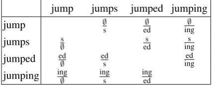
For our purposes, it is sufficient to interpret string differences as ordered pairs of strings.2 In its turn, left/right commonalitycan be defined as the longest common prefix/suffix of two strings. The left commonality of jumps and jumped is jump, and the right commonality ofundoandredoisdo. Given aparadigm (set of strings)P withn el-ements, its left/right self-difference array is the

n×n arrayD such thatD[i][j] is the left/right difference ofP[i]andP[j]. The array of common-alities is defined similarly. A paradigm isregular if each row in its self-difference array has a single common nominator and all elements in its com-monality array are identical (ignoring the main di-agonal).

jump jumps jumped jumping

jump ∅_{s ed}∅ _ing∅

jumps _∅s _eds _ings

jumped ed

∅ eds

ed ing

jumping ing_∅ ing_s ing_ed

Figure 1: Regular paradigm: right self-differences of{jump, jumps, jumped, jumping}

2_{AsGoldsmith(2011) points out, one can also think of}

the right difference ofsandtas afunctionthat mapsttos.

try tries tried trying

try _iesy _iedy _ing∅

tries ies_y s

d

ies ying

tried ied_y d_{s ying}ied

trying ing_∅ ying_ies ying_ied

Figure 2: Non-regular paradigm: right self-differences of{try, tries, tried, trying}

This notion of self-difference is still limited to prefixes and suffixes. LetP = {w1, ..., wn}be a paradigm whose left and right self-difference ar-rays are regular, withlandrdenoting its (unique) left and right commonality respectively. Omit-ting some details for the sake of space, we define the set of internal difference substrings of P as

{l−1w1r−1, ..., l−1wnr−1}.

Under the assumptions outlined previously, the task of identifying alternations reduces to finding segment-sized (or smaller) differences between re-alizations of the same morpheme. The following recursive definition captures this idea:

(14) Analternationis the set of internal differ-ence substrings of a paradigm that is reg-ular if any previously determined alterna-tions are ignored and, moreover, satisfies two conditions:

(i) the paradigm’s left or right common-ality is a non-empty string;

(ii) none of the difference substrings are longer than one character.

3.3 A two-step algorithm

In the input, morphs are arranged into sets by gloss tag, each morph forming its owngroup. A frag-ment of the input is shown below.

(15) Q:{[m7_{], [}m e_]}

PST:{[d7], [d e], [t7], [t e]}

P1PL:{[b e z], [e b e z], [7b7z]}

differences and making more alternations accessi-ble to subsequent passes. The algorithm alternates between extraction and reduction until the number of groups stops decreasing.

Consider the toy example in (15). The first it-eration starts out with no known alternations; the only morph set conforming to (14) isQ. The ex-traction step discovers one alternation:{e,7}. The reduction step then collapses all morph groups that are identical up to this alternation:

(16) Q:mm e7,

PST:d_{d e}7,, t_{t e}7,

P1PL:b e z, e b e z_7b7z,

At the second iteration (17), members of the {e,

7} set are now treated as the same segment, and

PSTandP1PLsatisfy the conditions of (14). They

yield two new alternations, {d, t} and {∅, e, 7}, allowing the reduction step to collapse both PST

andP1PL:

(17) Q:m_{m e}7,

PST:

("_d7,

d e,

t7,

t e

#)

P1PL: _∅

b e z,

e b e z,

7b7z

At this point no further reduction is possible, and the algorithm halts.

3.4 Intermediate results

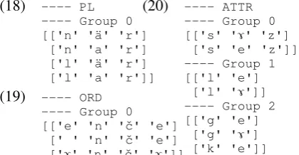
The Mishar Tatar sample contained 55 different gloss tags and 160 surface realizations. The algo-rithm converged after three iterations, collapsing the morphs into 85 groups.

Correct {d, n, t},{d, t},{∅, k, g},{l, n},

{k, g},{∅, e,7},{a, ¨a},{e,7}

Incomplete {∅,7},{∅, ¨a}

Incorrect {g, s},{n,N}

Table 2: Extracted alternations

The following output snippets illustrate the work of the reduction step. Multiple processes af-fecting the same morpheme can be learned (18); this also holds for alternations with zero (19). Not every set of morphs is reduced to a single group; the algorithm has successfully learned that the

ATTR gloss corresponds to three different attribu-tivizer suffixes, each of which has multiple real-izations (20).

(18) ---- PL ---- Group 0 [['n' '¨a' 'r']

['n' 'a' 'r'] ['l' '¨a' 'r'] ['l' 'a' 'r']]

(19) ---- ORD ---- Group 0 [['e' 'n' 'ˇc' 'e']

[' ' 'n' 'ˇc' 'e'] ['7' 'n' 'ˇc' '7']]

(20) ---- ATTR ---- Group 0 [['s' '7' 'z']

['s' 'e' 'z']] ---- Group 1 [['l' 'e']

['l' '7']] ---- Group 2 [['g' 'e']

['g' '7'] ['k' 'e']]

One interesting observation is related to the learner’s ability to retain group boundaries if the groups appear to represent distinct morphemes. This has a practical potential for detecting incon-sistencies in labelling – such as the COMP gloss tag being used for the complementizerdipand the comparative suffix -r{a¨a}k (21), when CMPR is expected for the latter (22).

(21) ---- COMP ---- Group 0 [['d' 'i' 'p']] ---- Group 1 [['r' '¨a' 'k']

['r' 'a' 'k']]

(22) ---- CMPR ---- Group 0 [['r' 'a' 'k']]

4 Learning contexts

4.1 Rules and locality

Above, we have introduced a method of detecting likely phonological processes and collecting them as sets of alternating segments. This section makes the next logical step and focuses on patterns gov-erning the distribution of alternants.

A straightforward way to formalize this task and define its boundaries is grounded in formal language theory. Two classes of subregular lan-guages are particularly relevant to the discussion of phonology. One of them is Strictly Local lan-guages (McNaughton and Papert 1971; Rogers and Pullum 2011). Given an alphabetΣ, a Strictly

intervening elements that do not belong to the sub-set.

How can this model be used to produce a practi-cal representation of a phonologipracti-cal process? One way is to link each alternant occurring in a sur-face form to a set oftrigger segments, indicating whether they occur to the left or right. Each al-ternation should also be associated with a set of transparent segments – non-tier elements in TSL terms. This is essentially abigram model, encod-ing dependencies between pairs of elements, and has a clear counterpart in 2-TSL grammars. Given an alternation withnvariants, the process of learn-ing the rule boils down to determinlearn-ing the direc-tionality and partitioning the set of segments into

n+ 1 subsets of triggers (for each alternant) and transparent segments.

4.2 Mutual information

Mutual information (MI) is a measure of depen-dence between two random variables, or the reduc-tion of uncertainty in one random variable through the other (Cover and Thomas 2012).

(23) MI(X;Y) = P

x∈X P y∈Y

p(x, y) log_2pp_(x(x,y_)p()_y)

For the task at hand, it is convenient to think of MI as the expected value ofpointwise mutual in-formation(PMI). In its turn, PMI is an indication of how much the probability of a particular pair of events differs from what it is expected to be as-suming independence (Bouma 2009). Intuitively, PMI measures correlation (positive or negative) between events.

(24) PMI(x;y) = log_2p(p_x(x,y_)p(y)₎

The PMI metric is naturally applicable to learning of vowel harmony. In our case, the algorithm is expected to learn the triggers and transparent seg-ments for each process, which translates into cal-culating PMI values with respect to each specific alternation. Instead of the full set of bigrams in the corpus, the input for this procedure is the set of bigrams containing an alternant (member of the alternation in question) and a context segment.

A character bigram can be defined either lo-cally, as a substringin a word, or nonlocally, as a subsequence (potentially non-contiguous pair), using left or right contexts of the alternant. These two parameters –localityanddirectionality– yield

four different modes of collecting bigrams; see Ta-ble3for a concrete example.

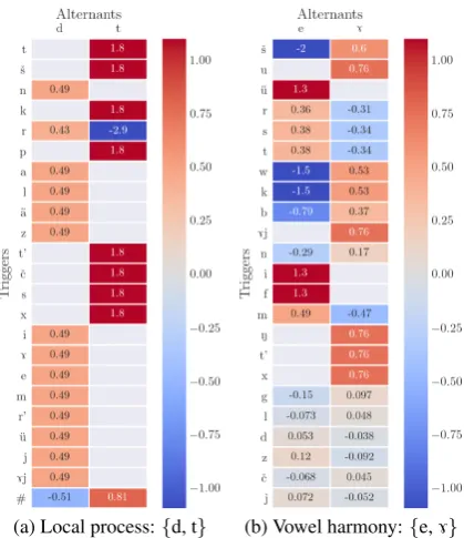
Left Right

Local ˇs7 7N

Nonlocal #7, b7, a7, ˇs7 7N,7#

Table 3: Bigrams for{e,7}in the wordbaˇs7N

Consider the voicing alternation {d, t} and the harmonic pair{e,7}. Both have triggers to the left of the target; the former is a local process, while the latter is nonlocal. Both alternations are present in the past tense suffix:

(25) a. ker-de enter-PST

b. k7ˇck7r-d7

shout-PST

c. 7r7ˇs-t7

scold-PST

d. teˇs-te fall-PST

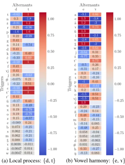
Presented in Figure3and Figure4are heat maps showing PMI values calculated for the alternations in question. High positive values in cells indicate attraction, whereas negative values correspond to elements repelling each other. Cells without val-ues indicate unattested bigrams.

(a) Local process:{d, t} (b) Vowel harmony:{e,7}

Figure 3: PMI heat maps for local left bigrams; higher values indicate stronger attraction between segments

very low PMI values. However, local bigrams do not perform well on the vowel harmony pair {e,

7}. Figure3bdoes indicate correct preference for some vowels, but the absolute values are compara-bly high for a number of consonants as well. With nonlocal bigrams the results are almost reversed. For {d, t} (Figure 4a), the pattern is obscured. However, nonlocal processes such as vowel har-mony yield some correct information: for {e, 7}

(Figure4b) more vowels and fewer consonants ex-hibit strong positive or negative correlation ten-dencies.

(a) Local process:{d, t} (b) Vowel harmony:{e,7}

Figure 4: PMI heat maps for nonlocal left bigrams

The heat maps demonstrate that PMI values can be successfully used to match triggers to alter-nants. What is needed at this point is a procedure that would assign correct sets of transparent seg-ments to each process – namely, the empty set for local processes and the set of consonants for vowel harmony.

Augmenting local bigrams with the notion of transparent segments produces a generalization applicable to both local and nonlocal processes. A left (right) local bigram consists of an alternant and the closest non-transparent segment to its left (right). One option, then, is to compare context segments directly in terms of how likely they are to be transparent for a given alternation. A non-transparent segment is expected to have high ab-solute PMI values – positive with the alternant it

triggers and negative with all other alternants. The definition of MI (23) can be rewritten as follows:

(26) MI= P x∈X

p(x) P y∈Y

p(y|x)PMI(x;y)

Fixingx and normalizing the value by its proba-bility to avoid unnecessarily high scores for rarely attested segments, we obtain the following metric:

(27) MI(x) = P y∈Y

p(x, y)PMI(x;y)

This allows torankcontext segments by their MI value. The bigrams have to be calculated in the nonlocal mode to capture information about long-distance dependencies. Intuitively, the higher a segment is ranked, the more likely it is to be trans-parent with respect to the alternation in question. For each segment, the ranking also shows the al-ternant that corresponds to the highest PMI value. The ranking for{e, 7}(left contexts) is shown in (28).

(28) ---- Alternation: {'e', '7'}:

N: 7 0.00001362

h: e 0.00001943

#: e 0.00003585

d: e 0.00004618

r: e 0.00004704

...

z: e 0.00034681

¨

o: e 0.00042929

o: 7 0.00051578

7j: 7 0.00051578

k: e 0.00053448

...

u: 7 0.01335405

i: e 0.01762960

¨

u: e 0.01845926

7: 7 0.03614305 ¨

a: e 0.03741840

e: e 0.04574272

a: 7 0.04901854

As expected, most vowels have high values, whereas consonants tend to score low. Some vow-els still end up in the middle – in particular,oand ¨o, which are uncharacteristic for this dialect and generally found in borrowed roots. Provided that the alternation set itself has been identified cor-rectly, for every trigger segment the highest PMI value unerringly points at the correct alternant un-less the segment is transparent.

4.3 Phonological viability and rule evaluation

phonological features come into play. Adopting the standard textbook definition, anatural classis a set of segments that share a particular value for some feature or a set of features (Odden 2013). A rule is consideredphonologically viablejust in case the sets of triggers of all alternants corre-spond to disjoint natural classes.34

Phonological viability introduces a straightfor-ward way of producing generalizations. Com-bined with PMI rankings, it can be used to gener-ate phonologically meaningful rules for known al-ternations. First, each trigger set is extended with segments in its natural class that have not occurred in the context of the given alternation. Second, any transparent segments that were accidentally added to the transparent list is removed from it if they are also found in one of the expanded trigger sets. These modifications producegeneralized rules.

We use two metrics to evaluate and compare these rules. The primary objective is to explain as many instances of the given alternation as pos-sible. This intuition is easy to formalize: an ex-ample is explained if it contains a correct trigger which is either adjacent to the alternant or sepa-rated only by transparent segments. Another op-tion is to calculate the average PMI over all (seg-ment, alternant) pairs, following the standard def-inition of mutual information shown in (24).

4.4 Assembling the pieces

In order to determine the best cutoff point in the ranking, each alternation A is processed as follows. At initialization, MI values are calcu-lated once with nonlocal bigrams in order to rank the segments; all subsequent calculations are per-formed with local bigrams. The set of transparent segments, TranspA, starts out empty. The algo-rithm traverses the ranking, starting with the low-est MI value. At each step, the selected segment is added toTranspA, and both metrics (mutual infor-mation and explained examples) are recalculated. Thus, TranspAis expanded incrementally until it

3

This is a simplification, as one of the trigger sets may form an unnatural class that corresponds to the general case – a fact captured by the Elsewhere Condition (Kiparsky 1973). The definition of phonological viability implements the Else-where Condition to some degree, as no natural class require-ment is imposed on the set of transparent segrequire-ments.

4

Under this definition, classes of segments specified by disjunction are generally unnatural. While languages have a tendency to favor natural classes (definable by feature con-junction) in their rules (Halle and Clements 1983), exploring more relaxed definitions for the purposes of determining ac-ceptable rules is an interesting avenue of future work.

contains all segments in the ranking; every step produces a new rule with triggers assigned accord-ing to the current PMI values. If the rule is phono-logically viable, it is converted into a generalized rule, and the metrics are recalculated once more. The procedure is performed twice for each alterna-tion, on left and right contexts separately. Once it halts, the best generalized rule is selected – which means that only phonologically viable configura-tions are eligible candidates.

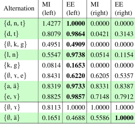
The results are summarized in Table4. For each alternation, MI and explained examples ratio (EE) are shown for the best rule based on left and right contexts. Colored rows indicate that the learner has both partitioned the set of attested context seg-ments and determined whether the trigger is to the left or to the right correctly with respect to the ground truth.

Alternation MI (left)

EE (left)

MI (right)

EE (right)

{d, n, t} 1.4277 1.0000 0.0000 0.0000

{d, t} 0.8079 0.9864 0.0421 0.3143

{∅, k, g} 0.4951 0.4909 0.0000 0.0000

{l, n} 0.5547 0.9738 0.0514 0.1154

{k, g} 0.0814 0.1653 0.0000 0.0000

{∅,7, e} 0.8431 0.6220 0.6205 0.5357

{a, ¨a} 0.8319 0.9733 0.8331 0.8387

{e,7} 0.8825 0.9857 0.7148 0.7912

{∅,7} 0.8113 1.0000 1.0000 1.0000

{∅, ¨a} 0.1651 0.4688 0.5586 1.0000

Table 4: Rule evaluation for correct and incomplete alternations

As mentioned in section 2, some alternations are involved in multiple processes. For instance,

{k, g} conflates two assimilation processes with different directionality, while {∅, 7, e} corre-sponds to a combination of a local and nonlocal processes. As expected, they have lower scores.

Figure 5: Final PMI heat map for vowel harmony:

{e,7}, left contexts

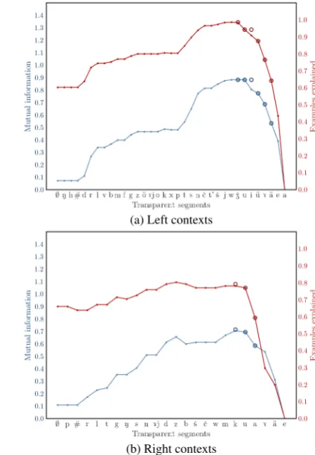
One way to gain insight into the procedure of context learning is to plot the step-by-step change of metric values depending on the set of transpar-ent segmtranspar-ents.

(a) Left contexts

(b) Right contexts

Figure 6: MI and explained examples for{t, d}

Figures6–7show graphs for left and right con-texts with respect to the{t, d}and{e,7} alterna-tions. Each graph has context segments, ordered according to the MI ranking, along its x-axis. Each point corresponds to a step performed by the al-gorithm – or, equivalently, to a rule whose set of transparent segments contains all items on the x-axis up to and including that point. In addition, circle markers are present at every phonologically viable step and indicate values obtained by gener-alized rules.

Graphs for local and nonlocal processes display strikingly different behaviour. The typical pic-ture for a local process is a monotonic sequence: both metrics start out high but decline steadily as more segments are declared transparent. For left-triggered processes, right contexts show notice-ably lower values throughout the procedure – es-pecially so if only phonologically viable steps are considered.

For vowel harmony (Figure7) the plots start low and show a distinct peak once a sufficient number of segments are moved to the transparent set. The peak corresponds to the last consonant in the rank-ing.

(a) Left contexts

(b) Right contexts

While the values for left contexts are still higher, the difference is not as great. This is an ex-pected result: since vowels serve as both triggers and targets of harmony, most vowels in non-final syllables would have a harmonizing vowel both to the left and to the right.

5 Discussion

This paper presents an approach to learning (mor-pho)phonological phenomena from small anno-tated datasets that combines information-theoretic methods with linguistic information. The proposal includes an algorithm that discovers phonologi-cal alternations (represented as sets of segments) shared by multiple morphological paradigms. The notion of mutual information is used to assign a set of contexts to each alternant. Possible rules are then restricted to phonologically plausible config-urations via a procedure reminiscent of regulariza-tion in machine learning. This approach is appli-cable to both local and nonlocal processes.

All these should be taken as interim results. One option for future work is to explore interaction be-tween alternation sets. For example, it may be possible to decompose the complex{∅, e, 7} al-ternation by first factoring out the known vowel harmony pattern{e,7}, leaving a simple local pro-cess. Other steps that follow directly from the re-sults described here include predicting and recon-structing morphs that are absent from the dataset and, as a more practically oriented goal, identify-ing inaccuracies and instances of mislabellidentify-ing in the data.

References

Diana Archangeli. 1988. Aspects of underspecification theory. Phonology, 5(2):183–207.

Gerlof Bouma. 2009. Normalized (pointwise) mutual information in collocation extraction. Proceedings of GSCL, pages 31–40.

Jan Baudouin de Courtenay. 1876. Rez’ja i rez’jane.

Slavjanskij sbornik, 3:223–371.

Thomas Cover and Joy Thomas. 2012. Elements of in-formation theory. John Wiley & Sons.

Gallagher Flinn. 2014. Modeling neutrality in Mongo-lian vowel harmony. Manuscript.

John Goldsmith. 2011. A group structure for strings: Towards a learning algorithm for morphophonol-ogy. Technical report, Technical Report TR-2011-06, Department of Computer Science, University of Chicago.

John Goldsmith and Jason Riggle. 2012. Information theoretic approaches to phonological structure: the case of finnish vowel harmony. Natural Language & Linguistic Theory, 30(3):859–896.

Morris Halle and George N. Clements. 1983. Prob-lem book in phonology: a workbook for introduc-tory courses in linguistics and in modern phonology. MIT Press.

Jeffrey Heinz, Chetan Rawal, and Herbert G. Tan-ner. 2011. Tier-based strictly local constraints for phonology. InProceedings of the 49th Annual Meet-ing of the Association for Computational LMeet-inguis- Linguis-tics, pages 58–64, Portland, Oregon, USA. Associa-tion for ComputaAssocia-tional Linguistics.

Paul Kiparsky. 1973. “Elsewhere” in phonology. In Paul. Kiparsky and Stephen R. Anderson, editors,

A festschrift for Morris Halle, pages 93–106. New York: Holt, Rinehart & Winston.

Robert McNaughton and Seymour Papert. 1971.

Counter-Free Automata. MIT Press.

MSU linguistic expedition. 1999–2012. Fieldwork ma-terials. Lomonosov Moscow State University.

David Odden. 2013. Introducing Phonology. Cam-bridge University Press.

Frans Plank. 1998. The co-variation of phonology with morphology and syntax: A hopeful history. Linguis-tic Typology, 2:195–230.

James Rogers and Geoffrey Pullum. 2011. Aural pat-tern recognition experiments and the subregular hi-erarchy. Journal of Logic, Language and Informa-tion, 20:329–342.

Lili Szab´o and C¸ agrı C¸ ¨oltekin. 2013. A linear model for exploring types of vowel harmony. Com-putational Linguistics in the Netherlands Journal, 3:174–192.

David Allen Wax. 2014. Automated grammar engi-neering for verbal morphology. Ph.D. thesis, Uni-versity of Washington.