Limitations of MT Quality Estimation Supervised Systems: The Tails Prediction Problem

Limitations of MT Quality Estimation Supervised Systems:

The Tails Prediction Problem

Erwan Moreau

CNGL and Computational Linguistics Group Centre for Computing and Language Studies School of Computer Science and Statistics

Trinity College Dublin Dublin 2, Ireland [email protected]

Carl Vogel

Computational Linguistics Group Centre for Computing and Language Studies

School of Computer Science and Statistics Trinity College Dublin

Dublin 2, Ireland [email protected] Abstract

In this paper we address the question of the reliability of the predictions made by MT Quality Estimation (QE) systems. In particular, we show that standard supervised QE systems, usually trained to minimize MAE, make serious mistakes at predicting the quality of the sentences in the tails of the quality range. We describe the problem and propose several experiments to clarify their causes and effects. We use the WMT12 and WMT13 QE Shared Task datasets to prove that our claims hold in general and are not specific to a dataset or a system.

1 Introduction

Machine Translation (MT) Quality Estimation (QE) has become an important subject of study in the past few years (Callison-Burch et al., 2012; Bojar et al., 2013). This follows directly from the erratic quality of MT output in general: although MT is now widely used in professional contexts, it is still prone to many errors; therefore a careful post-editing stage, performed by human experts, is usually needed. In this context, QE can help carrying out this process more efficiently, and more specifically to help in the decision process between the automatic and the manual stages: if a reliable indication of quality is provided for every machine-translated sentence, the human effort can be reduced. For example, a very bad translation is worthless because the translator usually has to spend more time fixing it than she or he would have spent translating the sentence from scratch; thus it makes more sense in such cases to either send the sentence back to an alternative MT system (e.g. trained on a different corpus), or simply leave it untranslated for the translator. Clearly the advantage of using a QE system depends on the reliability of its predictions. If it makes too many errors, then it only confuses the translation workflow; in this case the translators would perform better without it.

The quality of an (automatic) QE system cannot be perfect, but it should be at least controllable. That is, it should be possible to assess the reliability of the predictions made by a system, for instance by estimating the level of confidence of the predictions. Hopefully, QE systems will progress towards this kind of behaviour, but currently the evaluation methods are not entirely satisfactory from this perspective. In particular, after describing our experimental setting in§2, we will observe in§3 that the use of the Mean Absolute Error1_{(MAE) as a global evaluation measure hides huge discrepancies in the distribution} of errors among the range of scores. More precisely, supervised systems optimized to minimize the MAE have intrinsic flaws in the way they assess the tails of the quality range, i.e. the “very good” and the “very bad” sentences. In§4 we propose different ways to evaluate the impact of this problem, and also clarify what might be an important misunderstanding in what a QE system actually does (§4.2). Finally we propose in§5 several experiments: in§5.1 we show that the problem is not system-specific, and we test two ways to circumvent it in§5.2 and§5.3, but the price to pay in global performance is high.

This work is licensed under a Creative Commons Attribution 4.0 International Licence. Page numbers and proceedings footer are added by the organisers. Licence details:http://creativecommons.org/licenses/by/4.0/

1_{The MAE is defined as the mean over all instances of the absolute error, where the absolute error is the absolute value of}

the difference between the predicted and the actual value of the instance. Thus, the MAE score depends on the range of possible values (i.e., two datasets using different ranges cannot be compared).

2 Experimental Setup 2.1 Data

In this paper we use the three datasets from the WMT12 and WMT13 QE Shared Task (Callison-Burch et al., 2012; Bojar et al., 2013) which are intended to predict the quality of individual machine-translated sentences: the WMT12 task and the WMT13 task 1.1 and 1.3. The last two datasets are renamedwmt13a

andwmt13bin the rest of this paper. These three datasets differ by the way quality is measured:

• wmt12: effort scores, which have been assigned by three professional post-editors according to

predefined guidelines; scores range from 1: “the MT output is incomprehensible [..]” to 5: “the MT output is perfectly clear [..]”. The dataset was cleaned to avoid the cases with a high level of disagreement, and the scores were post-processed to harmonize the scale between the judges.

• wmt13a: HTER scores, which measure the distance between the MT output and the post-edited

sentence (Snover et al., 2006).

• wmt13b:post-editing time, that is, the time that the post-editor has spent correcting the MT output.

As a consequence, the set of scores have different characteristics: inwmt12, the distribution is highly discrete due to the integer values assigned by the judges. In wmt13athe distribution is more dense, whereas in wmt13b some values are spread extremely far from the mean.2 _{General statistics for the} datasets are given in table 1. In all datasets the input and MT output sentences are available to the system; the post-edited version of the sentences is also available, but it cannot be used by the QE systems (the test set post-edited sentences were provided only after the end of the task). We focus on predicting an absolute indication of quality rather than only ranking the sentences by quality; this is why we use the Mean Absolute Error (MAE) as the main evaluation measure rather than Spearman’s correlation or DeltaAvg (Callison-Burch et al., 2012).

2.2 Supervised QE System

In the observations and experiments described in this paper we use a QE system which follows a standard supervised learning approach: it was trained on the full training set for every task considered; when the performance on the training set is observed, it was assessed using 10-fold cross-validation (thus obtaining a prediction for every sentence in the train set based on a 90% subset). We have used Quest3_{(Shah et} al., 2013), an open-source tool for QE, to compute the 17 “black box features” which are also used in the WMT QE “baseline” system (see below). We have used Weka (Hall et al., 2009) (version 3.6.10), and after testing several options4 _{we found that using theSMOreg algorithm (Smola and Sch¨olkopf, 2004;} Shevade et al., 2000) with an RBF kernel5 _{was optimal with respect to the performance on the three} datasets.

We did not perform any feature selection or parameter tuning, because our main goal was to build a generic system. Additionally we favor the ease of reproducibility over optimal performance, which is out of the scope of this paper. We want our system to be as generic as possible (but still performing decently, of course), because we need it to be fairly representative of standard, state-of-the-art, supervised learning QE systems. This is very important, since our observations and experiments are supposed to generalize to the current most common approaches in QE.

Our task of making the system representative of state-of-the-art QE systems has been greatly facilitated by the fact that the organizers of the WMT12 and WMT13 QE Shared Task provide for every task the performance of a so-called “baseline system”. We can use exactly the same set of features and compare the results of our system against these obtained by this baseline system, which in turn does not deserve

2_{This is why we exclude the most striking outlier from the training set: 1115.906, line 294. The test set is left unchanged.}

3_{http://staffwww.dcs.shef.ac.uk/people/L.Specia/projects/quest.html– last verified 05/14.}

4_{In particular, M5P regression trees generally achieve nearly as good performance as SVM regression. We have also}

observed that at least the most important characteristics reported in this paper for an SVM system hold for M5P regression as well.

its name since it has actually always performed well in every task: it ranked 8th out of 20 in the WMT12 official ranking, 12th out of 17 in WMT13a, and 6th out of 14 in WMT13b (MAE ranking). Thus, we can simply check that our system performs as well as this baseline system to ensure that it is equivalent, and therefore probably reasonably similar to the other supervised systems submitted to the Shared Tasks which perform similarly.6 _{Table 1 shows that our system performs roughly the same as the baseline} system on the three datasets.

Range Statistics Performance (test set)

Dataset of Quality Train set Test set Our system Baseline system

values direction instances mean std. dev. instances mean std. dev. cor. MAE cor. MAE

wmt12 [1,5] → 1832 3.44 0.88 422 3.29 0.98 0.56 0.69 0.58 0.69

wmt13a [0,1] ← 2254 0.32 0.17 500 0.26 0.19 0.44 0.15 0.46 0.15

wmt13b [0,+ inf[ ← 802 95.6 84.2 284 116.9 108.3 0.70 50.9 0.70 51.9

Table 1: Datasets: statistics and performance. Quality direction: →means that the quality is better when the score is higher,←means the opposite; “cor.” is the Spearman’s correlation.

3 The Tails Prediction Problem

In this section we mostly observe the training set (using cross-validation), in order to dismiss the possi-bility that the observed phenomenon is caused by the differences in the distributions of scores between the training set and the test set. Since it is easier for a supervised learning algorithm to annotate some data from the set it was trained on than from a different dataset, problems which appear with the former are very likely to appear as well (possibly accentuated) with the latter.

2 3 4 5

1 2 3 4 5

gold

predict

(a) wmt12. Spearman cor.: 0.53

0.2 0.3 0.4 0.5

0.00 0.25 0.50 0.75 1.00

gold

predict

(b) wmt13a. Spearman cor.: 0.37

0 100 200

0 100 200 300 400 500

gold

predict

(c) wmt13b. Spearman cor.: 0.62

Figure 1: Scatter plots showing how predicted scores differ from gold scores (test set). Every point (X,Y) corresponds to one sentence for which X is the gold score and Y the predicted score. Darker areas correspond to more dense areas; the vertical and horizontal lines indicate the frontiers of 20%-quantiles for both variables (for instance, the points which are on the right side of the rightmost vertical line account for the 20% highest gold scores). Remark: a few outliers are not visible on the wmt13b plot (their gold scores are higher than 500, and their predicted scores are lower than 250).

Figure 1 shows that the points are very scattered and do not follow the diagonal very closely, but also that the range of predicted scores is significantly different from the range of gold scores: no sen-tence is predicted below 2 for wmt12, above 0.55 for wmt13a and above 260 for wmt13b, whereas the corresponding range of gold scores is much wider. Figure 2, which shows the distribution of gold vs. predicted scores for the training sets, gives a more precise picture of this difference: in all three datasets, the predicted scores tend to belong to a smaller set of values centered approximately around the mean. There are clearly more predicted values than gold values in this area, and this is confirmed by the much smaller standard deviation for the predicted scores.

It is possible to obtain a clearer picture by “flattening” the distribution, that is, instead of drawing histograms in which points with the same value (or a close value) are accumulated, we represent every

0 100 200 300

1 2 3 4 5

score

count

group gold predict

(a) wmt12.σG= 0.88, σP = 0.50 0 100 200 300 400

0.00 0.25 0.50 0.75 1.00

score

count

group gold predict

(b) wmt13a.σG= 0.17, σP = 0.07 0 50 100 150

0 200 400 600

score

count

group gold predict

(c) wmt13b.σG= 84.2, σP = 46.5

Figure 2: Combined distributions of the gold scores and predicted scoreson the training set for the three datasets.σG(resp.σP) is the standard deviation for gold (resp. predicted) scores.

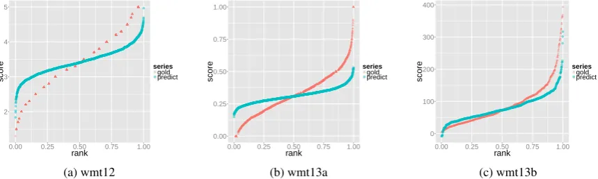
point on the X axis and sort the values on this axis, so that their actual value can be observed on the Y axis, as shown on figure 3. This figure shows that, in all three cases, the predicted scores are tightly clustered around the median, which is the point where the two curves cross each other. If the system predicted scores according to the distribution it observed on the training set, the two curves would be close; instead, they clearly diverge from each other as the distance to the median increases. This means that the model tends globally to overestimate the points below the median and, symmetrically, underestimate the points above the median (though the symmetry is degraded in 3c, since the range is unbound to the right).

In figure 3 the two sets of points are sorted independently: the sentence(x, y) on the curve of gold scores is different from the one with the samex on the curve of predicted scores. Yet this observation of “tightened” predicted scores cannot be fully understood without taking into account the risk of error in the prediction process, as it was visible on the scatter plots in figure 1. Thus it is also useful to look at the sorted scores, but with their corresponding predicted score (for the same sentence) plotted on the samexcoordinate; this what is shown on figure 4, for thewmt13adataset only (because the phenomenon is the most accentuated in this dataset, and scores conveniently belong to[0,1]). On figure 4a one can see that the set of predicted scores are mostly contained in a slightly inclined rectangle; clearly they do not follow the curve of gold scores, but here one can see why: the fact that there are many points at the same level on the Y axis along the whole X axis shows that the algorithm cannot make a clear distinction between the different levels of quality. For example, there are approximately as many scores predicted around 0.3 which correspond to actually very good (rank near 0) and very bad sentences (rank near 1). From a different perspective, figure 4b shows very clearly that the farther the gold score of a sentence is from the mean (0.32), the more likely it is to be predicted with a large error.

2 3 4 5

0.00 0.25 0.50 0.75 1.00

rank score series gold predict (a) wmt12 0.00 0.25 0.50 0.75 1.00

0.00 0.25 0.50 0.75 1.00

rank score series gold predict (b) wmt13a 0 100 200 300 400

0.00 0.25 0.50 0.75 1.00

rank score series gold predict (c) wmt13b

0.00 0.25 0.50 0.75 1.00

0.00 0.25 0.50 0.75 1.00

rank

score

group gold predict

(a)Gold scores as reference. Sentences are sorted by their gold score; the X axis gives their corresponding rank; the

predictedscore of a sentence is plotted on the same abscissa, thus showing both the gold (in red) and predicted score (in blue) of the sentence on the Y axis. The predicted scores which appear on the same vertical line correspond to different sentences which have the same (or very close) gold scores.

0.00 0.25 0.50 0.75 1.00

0.00 0.25 0.50 0.75 1.00

rank

score

group absErr gold

(b)Absolute error as reference. Sentences are sorted by their absolute error; the X axis gives their corresponding rank; thegoldscore of a given sentence is plotted on the same abscissa, thus showing both the error (in red) and gold score (in blue) of the sentence on the Y axis. The gold scores which appear on the same vertical line correspond to different sen-tences which have the same (or a very close) absolute error.

Figure 4:wmt13a, training set: sentences sorted by gold score (left) or absolute error (right).

The issue is constant among the datasets, but with a variable impact. To some extent, it could be summarized in the following way: it appears that the system does not try to predict the actual quality of the sentences, but instead applies a simple optimization strategy; since a large majority of sentences belong to a relatively small range of values in the middle of the full possible range of scores, predicting any score outside this range is taking a big risk. Consequently it is safer, in order to minimize the error rate, to ignore (or barely take into account) the rare cases which belong to the tails. Hence the system ends doing the opposite of what is usually expected from a quality estimation system: the most common cases are rather accurately recognized, but the most striking anomalies are left undetected or poorly labelled as such. This behaviour can be explained by the following reasons:7

• The supervised learning optimization criterion is very often the minimization of the MAE,8 as in our system. This leads the algorithm to favor the interval of scores where there are many instances, since their weight is more important in the average.

• The datasets are unbalanced, which is certainly realistic in terms of application, but it also en-courages the algorithm to assign scores in the interval which would be the “default class” in a classification problem; that is, without any clear indication in the features, it is strategically wiser to bet on the most probable answer.

• The risk is lower with respect to MAEto assign a score in the middle of the range of possible values rather than at the extremes. For instance if the range is[1,5]the maximum absolute error at 3 is 2, whereas it is 4 at 1 or 5. However, at least forwmt13a, the data shows that, if this hypothesis had a real impact, the predicted scores would be closer to 0.5 than to the mean 0.32.

4 Detecting and Evaluating the Tails Quality 4.1 Possible Measures

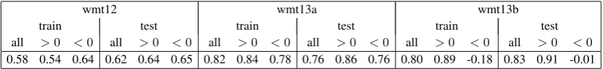
We propose below different measures intended to evaluate the impact of the tails prediction problem. Since it can be defined as an increased level of error for sentences which are far from the mean, a simple first measure is the correlation between the distance from the gold score to the mean and the absolute error: this value reflects whether the errors are higher in the tails than close to the mean and to what extent (in other words, it measures how strong the divergence observed on the right part of figure 4b is). Table 2 shows how high Pearson’s correlation is in our data.

A simple way to measure the performance locally in the tails is to consider the task as a binary classi-fication problem, as if we were only interested in recognizing whether a sentence belongs to a particular

wmt12 wmt13a wmt13b

train test train test train test

all >0 <0 all >0 <0 all >0 <0 all >0 <0 all >0 <0 all >0 <0 0.58 0.54 0.64 0.62 0.64 0.65 0.82 0.84 0.78 0.76 0.86 0.76 0.80 0.89 -0.18 0.83 0.91 -0.01

Table 2: Correlation between the absolute error and the distance to the mean of the gold score.

“>0” (resp. “<0”) is the correlation when taking only into account the scores above (resp. below) the mean; this gives a more precise picture for the top/bottom quality scores. For example, inwmt13bthe top quality (lowest) scores are very well predicted, as opposed to the bottom quality (highest) scores.

subset of scores. For example, the frontier between the classes can be fixed between the 90% lowest scores (negative) and the 10% highest (positive): it is then possible to observe the last 10% using the standard evaluation measures: precision (proportion of true positive among the sentences labeled as positive), recall (proportion of sentences labeled as positive among all positive sentences) and F1-score (harmonic mean of the precision and recall).9 _{The values of these measures are given for three} thresh-olds in table 3. As expected, the recall is extremely low in the tails; it is even 0 in most cases for the 5% threshold, which means that the system does not assign any score in the 5% top/bottom of the range observed on the training data.

Data+tail 5% 10% 20%

limit P R F1 limit P R F1 limit P R F1

wmt12 B ≤2.0 – 0.0 – ≤2.3 0.33 0.01 0.02 ≤2.7 0.73 0.16 0.26 T ≥5.0 – 0.0 – ≥4.7 0.50 0.02 0.04 ≥4.2 0.65 0.18 0.28 wmt13a B ≥0.62 – 0.0 – ≥0.54 – 0.0 – ≥0.47 0.62 0.11 0.19 T ≤0.06 – 0.0 – ≤0.11 – 0.0 – ≤0.17 0.50 0.01 0.01 wmt13b B ≥272 – 0.0 – ≥186 0.76 0.26 0.39 ≥134 0.71 0.43 0.54 T ≤18.2 0.5 0.05 0.09 ≤24.8 0.18 0.06 0.10 ≤35.7 0.52 0.30 0.38

Table 3: Local classification measures (test set). “T” (resp. “B”) refers to the top (resp. bottom) quality tail; P/R/F1 are the standard Precision/Recall/F1-score.10 _{Example: 10% of the scores for the}

wmt12training data are higher than 4.7 (top quality tail); among the gold scores in the test set which are

higher than this 4.7 threshold, only 2% are predicted as higher than 4.7 (recall); and among the scores predicted as higher than 4.7, exactly 50% are actually higher than 4.7 (precision).

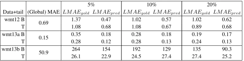
Additionally, we have separately proposed a measure which aims to evaluate the ranking error locally (Moreau and Vogel, 2013). The same idea can be applied to scoring errors: the Local MAE (LMAE) can be computed on a particular range of scores. The difference with global MAE is that, for a given sentence, the gold score or the predicted score can belong to the range while the other does not. This is why there are two versions of this measure: gold-based LMAE and prediction-based LMAE, which, as their names suggest, take into account only the gold scores (resp. predicted scores) which belong to the range in the absolute difference|gold−predicted|, as defined in definition 4.1.

Definition 1(Local MAE (LMAE)). LetS be a set of sentences, andDthe interval of possible scores:

9_{In the observations which follow we choose to set the limits (5%, etc.) based on the training set even though the test set}

is observed. In other words, the absolute score corresponding to the percentage is calculated using the training set gold scores, which might differ from the value calculated from the test set. The disadvantage is that the number of values in the test set in the corresponding range does not necessarily correspond to the percentage, but this way the limits do not depend on the test set, so that values obtained on different test sets would be comparable.

10_{We consider theN% limits computed from the range of gold scores, and not from the range of predicted scores: this makes}

for every sentences∈S,predicted(s)∈D, gold(s)∈D. For any subintervalI ⊆D:11

LMAEgold=mean n gold(s)−predicted(s) ssuch thatgold(s)∈I

o

LMAEpred=mean n gold(s)−predicted(s) ssuch thatpredicted(s)∈I

o

To some extent, the gold-based LMAE (resp. prediction-based) is similar to a recall measure (resp. precision) because it takes into account the true positive and the false negative (resp. the true positive and the false positive) with respect to the range. This can be observed in table 4, which gives the values of these two measures for three thresholds on the three datasets:LMAEgoldis almost always much higher

than the global MAE, whereas thereLMAEpredis often close to or lower than the global MAE. This is

because, compared to the gold scores, the top or bottom predicted scores are closer to the centre of the range. Therefore the sentences taken into account include some actual “tails sentences” (for which the absolute error is high), but they can also contain many sentences which actually belong to the area (for which the absolute error is low).

5% 10% 20%

Data+tail (Global) MAE LMAEgold LMAEpred LMAEgold LMAEpred LMAEgold LMAEpred

wmt12 B _0.69 1.37 0.47 1.02 0.57 1.02 0.62

T 1.08 0.68 1.08 0.67 0.89 0.68

wmt13a B _0.15 0.35 0.18 0.28 0.18 0.19 0.17

T 0.28 0.12 0.28 0.13 0.24 0.13

wmt13b B _50.9 264 154 192 129 135 90.3

T 26.1 22.9 24.5 27.4 27.4 25.2

Table 4: Local MAE evaluation (test set). “T” (resp. “B”) refers to the top (resp. bottom) quality tail. Example: for the wmt13b data, among the 10% actual top quality sentences (i.e. the 10% lowest gold scores), the mean absolute error is 26.1. This is lower than the global MAE (50.9), as opposed to all the other cases; this confirms that the top quality tail in wmt13bis particularly well predicted (this is certainly a consequence of the strongly skewed distribution in this dataset).

4.2 The Post-edited Sentences Test

A good way to evaluate the discrepancies in the reliability of the quality scores in the tails is to apply the QE system to a set of very good or very bad sentences. Thankfully the post-edited versions of the sentences were provided with the WMT datasets; since by definition their quality is perfect, they make a perfect case for such a test.12 _{In theory, all these sentences should be assigned a score close to top} quality.13 _{For every dataset we run the same QE system, i.e., we compute the features for the post-edited} sentences using Quest, then apply the model built with the regular training data to these features. We tried with both the post-edited version of the training set and test set, when provided.14

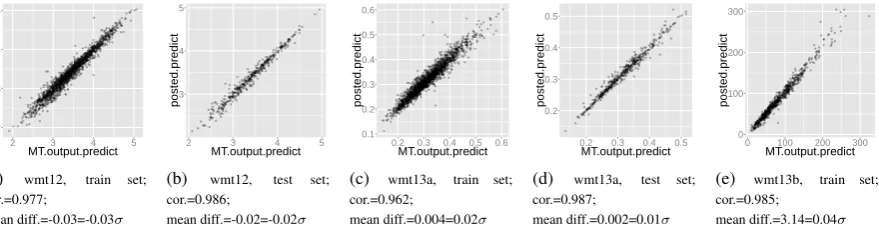
Our original goal was to observe how high the error rate was globally, but it turned out that the pre-dicted scores follow a distribution which is very similar to the one followed by the MT output (the means are very close as well, which implies that the MAE is very high). This led us to observe how the MT out-put scores and the post-edited version scores are correlated. In most cases the two scores are very close, as shown on figure 5. This is obviously a very serious issue, since it means that, in general, the system is not able to distinguish between a sentence which needs correction and the same sentence after correction.

11_{Remark: ifI=D,LMAE}

gold=LMAEpred=MAE.

12_{Independent assessment of the post-edited sentences is, of course, not guaranteed to yield the judgement that they would}

not benefit from further editing, though.

13_{That is, 5 for thewmt12dataset and 0 for thewmt13adataset (since HTER scores measure the distance against the}

post-edited version, and here we compare the post-post-edited sentence against itself); thewmt13bdataset is based on post-edited time, so there is no exact value corresponding to perfect sentences but the scores should very low.

2 3 4 5

2 3 4 5

MT.output.predict

posted.predict

(a) wmt12, train set; cor.=0.977;

mean diff.=-0.03=-0.03σ 3 4 5

2 3 4 5

MT.output.predict

posted.predict

(b) wmt12, test set; cor.=0.986;

mean diff.=-0.02=-0.02σ

0.1 0.2 0.3 0.4 0.5 0.6

0.2 0.3 0.4 0.5 0.6

MT.output.predict

posted.predict

(c) wmt13a, train set; cor.=0.962;

mean diff.=0.004=0.02σ

0.2 0.3 0.4 0.5

0.2 0.3 0.4 0.5

MT.output.predict

posted.predict

(d) wmt13a, test set; cor.=0.987;

mean diff.=0.002=0.01σ

0 100 200 300

0 100 200 300

MT.output.predict

posted.predict

(e) wmt13b, train set; cor.=0.985;

mean diff.=3.14=0.04σ

Figure 5:MT output predicted scores vs. post-edited predicted scores“mean diff.” is the mean of the difference between the post-edited score and the MT output score; it is also expressed as a multiple ofσ, whereσis the standard deviation of the MT output gold scores (specific to each particular dataset).

It is however able to see a slight difference at the document level: we have performed a paired Student’s test for each dataset, which shows that the mean of the scores predicted for the post-edited sentences is significantly lower in the wmt12case and higher in the wmt13aand wmt13bcases (as expected by the definition of scores) than the scores predicted for the MT output sentences. Nevertheless, the mean difference is extremely low (see figure 5), never higher than 0.04 standard deviations.

Furthermore, there is no visible impact of the quality of the MT output, although one would expect the correlation to be lower for low quality sentences: by definition, there are more differences between the MT output and the post-edited version for these sentences, so it should be easier for the system to detect the different level of quality between the two. In other words, it is quite understandable that the system does not detect the difference for an MT output of relatively good quality, but the fact the post-edited version of the really bad translations are also rated as really bad is a major issue. It must be remembered that we are not refering to a flaw solely in our own system, but nearly across the board in the state of the art systems.

These observations, which hold for every dataset, show that QE systems do not capture the actual quality of the sentences: instead, it seems that what they measure is probably thedifficulty of

machine-translating a sentence. Indeed, the set of Quest features that we use contains many features which depend

only on the source sentences. Moreover, this conclusion is consistent with the fact that Bic¸ici et al. (2013) obtain very good results on the WMT12 dataset using only the source sentences.

Explaining this observation with precision would require a more detailed analysis which is out of the scope of this paper. Nevertheless, it is fairly clear that the features which are used fail to capture the subtlety and/or the diversity of the difference between a faulty sentence and its corrected version; this might be because a single sentence does not offer enough clues for the system to make such a fine-grained distinction, in which case it would be necessary to rethink the definition of the QE problem.

In other work, we examine linguistic quality of items in relation to reference corpora (Moreau and Vogel, 2013;?). By comparison to the supervised learning studied here, such work is weakly supervised since there is no use of absolute scores. This yields a version of the QE problem that may be deemed too relativistic, but does represent an alternative approach. Unfortunately, because of the very difference in the use of absolute scores, they cannot be directly compared on this. Thus, we focus here on empirical exploration of the nature of the problem in estimating quality in the case of supervised learning.

5 Experiments

In this section we devise several experiments intended to explore different aspects of the problem in more detail. In particular, we try to evaluate the impact of the possible causes described in§3: first we show in§5.1 that it affects most QE systems, especially those optimized to minimize MAE. Then in§5.2 and

5.1 Tails Prediction for WMT12 Participating Systems

In order to test if the tails prediction problem is general to most supervised QE systems, we apply the local performance measures to the scores predicted on the test set by the participating systems in WMT12.15 Table 5 shows some detailed results for the four best systems at WMT12. It confirms that the predictions made for the tails are generally significantly worse than they are globally, and especially that the systems tend to predict very few values at the ends of the range of values: recall in the 10% bottom or top scores is never higher than 12%.16 _{It is also worth noticing that the first system, which performs significantly} better than the others, is the only one which was not optimized to minimize the MAE but to maximize the DeltaAvg score (Soricut et al., 2012). In particular, this system obtains a recall higher than the others in most cases (especially in the 5% and 10% tails), which is certainly due to the fact that it assigns more scores far from the mean (in other words, this system takes more risk). This tends to confirm our hypothesis that the minimization of the MAE as learning criterion is one of the causes of the problem.

Correlation Bottom Top

System ID Global dist.mean. 5% 10% 20% 5% 10% 20%

MAE vs abs.err. R G-LMAE R G-LMAE R G-LMAE R G-LMAE R G-LMAE R G-LMAE

SDLLW M5PbestDeltaAvg 0.61 0.49 0.05 1.02 0.07 0.76 0.32 0.76 0.02 0.96 0.12 0.99 0.26 0.84

UU best 0.64 0.53 0.0 1.21 0.07 0.91 0.26 0.91 0.0 1.02 0.04 1.01 0.22 0.81

SDLLW SVM 0.64 0.55 0.0 1.33 0.0 0.98 0.17 0.98 0.02 0.89 0.06 0.91 0.32 0.75

UU bltk 0.64 0.58 0.0 1.22 0.06 0.91 0.27 0.91 0.0 1.07 0.02 1.05 0.27 0.83

Table 5: Tails prediction quality for the 4 best systems at WMT12 (test set). The second column contains the correlation between the distance to the mean and the absolute error; the columns R and G-LMAE contain respectively the recall and the gold-based local MAE scores (see§4.1).

5.2 Adding the Post-edited Sentences to the Training Set

In this experiment we use the post-edited sentences again (see§4.2), but this time adding them to the training set in order to observe the impact on the test set.17 _{These instances are progressively added to} the official training set (in random order). We focus on the top quality tail, since it is the one which is expected to benefit from adding sentences with top scores to the training set. Figure 6 shows how the local MAE scores improve as post-edited instances are added. Only the gold-based LMAE scores are represented, because these provide a recall-like information and the observations show that recall (in the tails) is the main weakness of QE systems (see§4.1).

As expected, in all cases adding top quality sentences to the training set makes the system decrease the error rate in the top quality tail. Of course this local improvement comes at the price of degrading the global performance, although for thewmt13adataset (fig. 6b) the global error even improves until almost half of the sentences have been added. In the case of thewmt13bdataset (fig. 6c), since the QE system was already very good in predicting the top quality sentences (the LMAE is even better than the global MAE), the improvement is smaller and proportionally more costly for the global performance.

5.3 Balancing the Training Set

In this final experiment, we resample the training set (with replacement), in order to balance the gold scores over the full range of values. Since we can only use the discrete gold scores provided with the original training set, we compute a (random) uniform distribution but select the closest available score (randomly picking an instance among those with this score). The resulting distribution is not uniform, and the training set contains many duplicate instances; therefore, the resulting training set is unlikely to yield very good results in general, but it is no longer subject to the “statistical attraction” towards the mean that we have observed.

15_{These values were kindly provided by the organizers of the WMT12 QE Shared Task.}

16_{This is true for all but 3 participating systems, and these exceptions correspond to systems which performed worse globally.} 17_{We assign perfect scores to all these sentences: 5 forwmt12, 0 forwmt13a; forwmt13b, we use the mean of the time spent}

● ●● ●● ●● ● ● ●● ● ● ● ● ●●●● ● ● ●● ●● ● ● ● ●● ● ●● ● ● ● ●●● ● 0.4 0.8 1.2

0% 25% 50% 75% 100%

sentences LMAE proportion ●0.05 0.1 0.2 global (a) wmt12. ●● ●●● ●● ● ● ● ●● ● ● ● ● ● ● ● ● ● ● ● ● ● ● ● ● ●● ●● ● ●●●● ● ●● 0.1 0.2

0% 25% 50% 75% 100%

sentences LMAE proportion ●0.05 0.1 0.2 global (b) wmt13a. ● ● ● ● ● ● ● ● ● ● ●● ● ●● ● ● ●● ●_{● ● ● ● ● ● ●● ● ● ● ● ●} ● ● ● ● ● ● ● 20 40 60 80

0% 25% 50% 75% 100%

sentences LMAE proportion ●0.05 0.1 0.2 global (c) wmt13b.

Figure 6: Improvement of gold-based LMAE as post-edited sentences are added to the train set.

Example: inwmt12, the gold-based LMAE for the top 20% sentences is higher than 0.8 when the system is trained only on the official train set (0% of the post-edited sentences added), but reaches 0.4 when about half of the post-edited sentences are added to the training set. However the global MAE (which takes all the sentences into account) increases from 0.7 (0%) to 0.9 (50% of the post-edited sentences added): since the system assigns more scores in the top tail, it makes larger errors globally. Remark: the MAE and LMAE values are measured on the same set of sentences for every percentage on the X axis.

The model obtained from the balanced training set has been applied to the original test set. Table 6 gives the local results observed in the tails: in most cases, the recall increases drastically compared to using the regular training set, or is at least identical,18_{causing a great increase in the F1-scores as well.} The LMAE scores do not show such an improvement, in fact the mean error is often higher than with the regular training set. This is due to the fact that the system is forced to assign scores far from the “easy cases” around the mean, therefore makes much bigger mistakes than in the previous case. As expected, the global MAE scores forwmt13aandwmt13bare much higher than the original MAE values (0.27 and 110.7 respectively, i.e. about twice the original values). Interestingly, the MAE stays almost constant (0.71 instead of 0.69) forwmt12. The correlation between the distance to the mean and the mean absolute decreases to 0.42, 0.05 and 0.26 forwmt12,wmt13aandwmt13b, respectively.

Classification measures Local MAE measures

Data+tail 5% 10% 20% 5% 10% 20%

limit P R F1 limit P R F1 limit P R F1 gold pred. gold pred. gold pred. wmt12 B ≤2.0 0.31 0.18 0.23 ≤2.3 0.49 0.20 0.28 ≤2.7 0.66 0.46 0.54 0.94 0.82 0.73 0.75 0.73 0.67 T ≥5.0 – 0.0 – ≥4.7 0.50 0.02 0.04 ≥4.2 0.69 0.19 0.29 1.28 0.72 1.26 0.65 1.07 0.71 wmt13a B ≥0.62 0.15 0.70 0.24 ≥0.54 0.17 0.75 0.28 ≥0.47 0.21 0.83 0.33 0.14 0.60 0.13 0.55 0.14 0.49 T ≤0.06 – 0.0 – ≤0.11 – 0.0 – ≤0.17 0.67 0.02 0.04 0.58 0.11 0.57 0.14 0.44 0.15 wmt13b B ≥272 0.15 0.55 0.23 ≥186 0.27 0.78 0.41 ≥134 0.38 0.91 0.54 156 243 118 235 101 199 T ≤18.2 0.20 0.20 0.20 ≤24.8 0.30 0.19 0.24 ≤35.7 0.55 0.26 0.35 128 61 114 45 110 41

Table 6: Local evaluation of the test set using a balanced training set. Cells in bold show an im-provement over the corresponding value with the original training set, as given in tables 3 and 4. The classification limits were computed on the original training set.

6 Conclusion and Future Work

To conclude, we have shown that there are very serious issues with the way supervised QE systems are built: they tend to be unable to reliably evaluate both the worst and the best quality sentences. Furthermore, they cannot distinguish between a faulty MT output sentence and its post-edited version. We have also shown that it is possible to improve the detection of the best/worst sentences by altering the distribution of the training set; however the question whether this can be achieved while maintaining a decent level of global performance remains open. But even if the cost in global performance is high,

18_{The only exception is the 20% top quality recall of the wmt13b dataset. This is certainly due to the very particular}

the techniques that we have tested could be useful in some specific applications of QE (for example, if the recall in the tails is more important than the precision).

We think that these observations raise questions about the definition of the QE problem. It might actually be necessary to define different kinds of QE tasks: depending on the targeted application (e.g. estimating post-editing time, retraining the MT model, discarding the worst sentences, etc.), there could be a specific setting which is more appropriate in terms of supervised/unsupervised learning, evaluation measure, precision/recall trade-off, etc. For instance, minimizing the MAE does not seem compatible with detecting anomalies, but might be relevant for estimating the cost of post-editing. Similarly, under the hypothesis that the sentence level is not sufficiently rich in information in order to obtain accurate predictions, an intermediate level of granularity might be considered (e.g. at paragraph level).

Finally, another great challenge with respect to the reliability of QE systems is their consistency when applied to different test sets, or more generally their dependency on the training set: in the perspective of applications, it is very important to know what level of confidence can be expected when applying a QE system or model to a new document.

Acknowledgements

We are grateful to Lucia Specia, Radu Soricut and Christian Buck, the organizers of the WMT 2012 and 2013 Shared Task on Quality Estimation, for releasing all the data related to the competition, including post-edited sentences, features sets, etc.

This research is supported by Science Foundation Ireland (Grant 12/CE/I2267) as part of the Centre for Next Generation Localisation (www.cngl.ie) funding at Trinity College, University of Dublin.

The graphics in this paper were created with R(R Core Team, 2012), using the ggplot2 library (Wickham, 2009).

References

Ergun Bic¸ici, Declan Groves, and Josef Genabith. 2013. Predicting sentence translation quality using extrinsic

and language independent features. Machine Translation, 27(3-4):171–192.

Ondrej Bojar, Christian Buck, Chris Callison-Burch, Christian Federmann, Barry Haddow, Philipp Koehn, Christof Monz, Matt Post, Radu Soricut, and Lucia Specia. 2013. Findings of the 2013 Workshop on Statistical Machine

Translation. InEighth Workshop on Statistical Machine Translation, WMT-2013, pages 1–44, Sofia, Bulgaria.

Chris Callison-Burch, Philipp Koehn, Christof Monz, Matt Post, Radu Soricut, and Lucia Specia. 2012. Findings

of the 2012 workshop on statistical machine translation. InProceedings of the Seventh Workshop on Statistical

Machine Translation, Montreal, Canada, June. Association for Computational Linguistics.

M. Hall, E. Frank, G. Holmes, B. Pfahringer, P. Reutemann, and I.H. Witten. 2009. The weka data mining

software: an update.ACM SIGKDD Explorations Newsletter, 11(1):10–18.

Erwan Moreau and Carl Vogel. 2013. Weakly supervised approaches for quality estimation.Machine Translation,

27(3):pp 257–280, September.

R Core Team, 2012. R: A Language and Environment for Statistical Computing. R Foundation for Statistical

Computing, Vienna, Austria. ISBN 3-900051-07-0.

Kashif Shah, Eleftherios Avramidis, Ergun Bic¸ici, and Lucia Specia. 2013. Quest - design, implementation and

extensions of a framework for machine translation quality estimation. Prague Bull. Math. Linguistics, 100:19–

30.

S.K. Shevade, SS Keerthi, C. Bhattacharyya, and K.R.K. Murthy. 2000. Improvements to the SMO algorithm for

SVM regression. Neural Networks, IEEE Transactions on, 11(5):1188–1193.

A.J. Smola and B. Sch¨olkopf. 2004. A tutorial on support vector regression.Statistics and computing, 14(3):199–

222.

Matthew Snover, Bonnie Dorr, Richard Schwartz, Linnea Micciulla, and John Makhoul. 2006. A study of

transla-tion edit rate with targeted human annotatransla-tion. InIn Proceedings of Association for Machine Translation in the

Radu Soricut, Nguyen Bach, and Ziyuan Wang. 2012. The SDL Language Weaver systems in the WMT12

Quality Estimation shared task. InProceedings of the Seventh Workshop on Statistical Machine Translation,

pages 145–151, Montr´eal, Canada, June. Association for Computational Linguistics.