On Dual Decomposition and Linear Programming Relaxations for Natural Language Processing

On Dual Decomposition and Linear Programming Relaxations

for Natural Language Processing

Alexander M. Rush David Sontag Michael Collins Tommi Jaakkola

MIT CSAIL, Cambridge, MA 02139, USA

{srush,dsontag,mcollins,tommi}@csail.mit.edu

Abstract

This paper introducesdual decompositionas a framework for deriving inference algorithms for NLP problems. The approach relies on standard dynamic-programming algorithms as oracle solvers for sub-problems, together with a simple method for forcing agreement be-tween the different oracles. The approach provably solves a linear programming (LP) re-laxation of the global inference problem. It leads to algorithms that aresimple, in that they use existing decoding algorithms;efficient, in that they avoid exact algorithms for the full model; and often exact, in that empirically they often recover the correct solution in spite of using an LP relaxation. We give experimen-tal results on two problems: 1) the combina-tion of two lexicalized parsing models; and 2) the combination of a lexicalized parsing model and a trigram part-of-speech tagger.

1 Introduction

Dynamic programming algorithms have been re-markably useful for inference in many NLP prob-lems. Unfortunately, as models become more com-plex, for example through the addition of new fea-tures or components, dynamic programming algo-rithms can quickly explode in terms of computa-tional or implementacomputa-tional complexity.1 As a re-sult, efficiency of inference is a critical bottleneck for many problems in statistical NLP.

This paper introduces dual decomposition

(Dantzig and Wolfe, 1960; Komodakis et al., 2007) as a framework for deriving inference algorithms in NLP. Dual decomposition leverages the observation that complex inference problems can often be decomposed into efficiently solvable sub-problems. The approach leads to inference algorithms with the following properties:

1_{The same is true for NLP inference algorithms based on} other exact combinatorial methods, for example methods based on minimum-weight spanning trees (McDonald et al., 2005), or graph cuts (Pang and Lee, 2004).

• The resulting algorithms are simple and efficient, building on standard dynamic-programming algo-rithms as oracle solvers for sub-problems,2 to-gether with a method for forcing agreement be-tween the oracles.

• The algorithms provably solve a linear program-ming (LP) relaxation of the original inference problem.

• Empirically, the LP relaxation often leads to an exact solution to the original problem.

The approach is very general, and should be appli-cable to a wide range of problems in NLP. The con-nection to linear programming ensures that the algo-rithms provide a certificate of optimality when they recover the exact solution, and also opens up the possibility of methods that incrementally tighten the LP relaxation until it is exact (Sherali and Adams, 1994; Sontag et al., 2008).

The structure of this paper is as follows. We first give two examples as an illustration of the ap-proach: 1) integrated parsing and trigram part-of-speech (POS) tagging; and 2) combined phrase-structure and dependency parsing. In both settings, it is possible to solve the integrated problem through an “intersected” dynamic program (e.g., for integra-tion of parsing and tagging, the construcintegra-tion from Bar-Hillel et al. (1964) can be used). However, these methods, although polynomial time, are sub-stantially less efficient than our algorithms, and are considerably more complex to implement.

Next, we describe exact polyhedral formula-tions for the two problems, building on connec-tions between dynamic programming algorithms and marginal polytopes, as described in Martin et al. (1990). These allow us to precisely characterize the relationship between the exact formulations and the

2

More generally, other exact inference methods can be used as oracles, for example spanning tree algorithms for non-projective dependency structures.

LP relaxations that we solve. We then give guaran-tees of convergence for our algorithms by showing that they are instantiations of Lagrangian relaxation, a general method for solving linear programs of a particular form.

Finally, we describe experiments that demonstrate the effectiveness of our approach. First, we con-sider the integration of the generative model for phrase-structure parsing of Collins (2003), with the second-order discriminative dependency parser of Koo et al. (2008). This is an interesting problem in its own right: the goal is to inject the high per-formance of discriminative dependency models into phrase-structure parsing. The method uses off-the-shelf decoders for the two models. We find three main results: 1) in spite of solving an LP relax-ation, empirically the method finds an exact solution on over 99% of the examples; 2) the method con-verges quickly, typically requiring fewer than 10 it-erations of decoding; 3) the method gives gains over a baseline method that forces the phrase-structure parser to produce the same dependencies as the first-best output from the dependency parser (the Collins (2003) model has an F1 score of 88.1%; the base-line method has an F1 score of 89.7%; and the dual decomposition method has an F1 score of 90.7%).

In a second set of experiments, we use dual de-composition to integrate the trigram POS tagger of Toutanova and Manning (2000) with the parser of Collins (2003). We again find that the method finds an exact solution in almost all cases, with conver-gence in just a few iterations of decoding.

Although the focus of this paper is on dynamic programming algorithms—both in the experiments, and also in the formal results concerning marginal polytopes—it is straightforward to use other com-binatorial algorithms within the approach. For ex-ample, Koo et al. (2010) describe a dual decompo-sition approach for non-projective dependency pars-ing, which makes use of both dynamic programming and spanning tree inference algorithms.

2 Related Work

Dual decomposition is a classical method for solv-ing optimization problems that can be decomposed into efficiently solvable sub-problems. Our work is inspired by dual decomposition methods for infer-ence in Markov random fields (MRFs) (Wainwright

et al., 2005a; Komodakis et al., 2007; Globerson and Jaakkola, 2007). In this approach, the MRF is de-composed into sub-problems corresponding to tree-structured subgraphs that together cover all edges of the original graph. The resulting inference algo-rithms provably solve an LP relaxation of the MRF inference problem, often significantly faster than commercial LP solvers (Yanover et al., 2006).

Our work is also related to methods that incorpo-rate combinatorial solvers within loopy belief prop-agation (LBP), either for MAP inference (Duchi et al., 2007) or for computing marginals (Smith and Eisner, 2008). Our approach similarly makes use of combinatorial algorithms to efficiently solve sub-problems of the global inference problem. However, unlike LBP, our algorithms have strong theoretical guarantees, such as guaranteed convergence and the possibility of a certificate of optimality. These guar-antees are possible because our algorithms directly solve an LP relaxation.

Other work has considered LP or integer lin-ear programming (ILP) formulations of inference in NLP (Martins et al., 2009; Riedel and Clarke, 2006; Roth and Yih, 2005). These approaches typically use general-purpose LP or ILP solvers. Our method has the advantage that it leverages underlying struc-ture arising in LP formulations of NLP problems. We will see that dynamic programming algorithms such as CKY can be considered to be very effi-cient solvers for particular LPs. In dual decomposi-tion, these LPs—and their efficient solvers—can be embedded within larger LPs corresponding to more complex inference problems.

3 Background: Structured Models for NLP

We now describe the type of models used throughout the paper. We take some care to set up notation that will allow us to make a clear connection between inference problems and linear programming.

Our first example is weighted CFG parsing. We assume a context-free grammar, in Chomsky normal form, with a set of non-terminalsN. The grammar contains all rules of the formA → B C andA →

Given a sentence withnwords,w1, w2, . . . wn, a

parse tree is a set of rule productions of the form

hA → B C, i, k, ji where A, B, C ∈ N, and

1 ≤ i ≤ k < j ≤ n. Each rule production rep-resents the use of CFG ruleA → B C where non-terminalA spans words wi. . . wj, non-terminal B spans words wi. . . wk, and non-terminal C spans wordswk+1. . . wj. There areO(|N|3n3)such rule productions. Each parse tree corresponds to a subset of these rule productions, of sizen−1, that forms a well-formed parse tree.3

We now define theindex setfor CFG parsing as

I={hA→B C, i, k, ji: A, B, C∈N,

1≤i≤k < j≤n}

Each parse tree is a vector y = {yr : r ∈ I}, withyr = 1if rule r is in the parse tree, andyr =

0 otherwise. Hence each parse tree is represented as a vector in{0,1}m_{, wherem = |I|. We useY} to denote the set of all valid parse-tree vectors; the set Y is a subset of{0,1}m _{(not all binary vectors} correspond to valid parse trees).

In addition, we assume a vector θ = {θr : r ∈

I}that specifies a weight for each rule production.4 Eachθrcan take any value in the reals. The optimal parse tree isy∗ = arg maxy∈Y y·θwherey·θ= P

ryrθris the inner product betweenyandθ. We useyrandy(r)interchangeably (similarly for

θr and θ(r)) to refer to ther’th component of the vector y. For example θ(A → B C, i, k, j) is a weight for the rulehA→B C, i, k, ji.

We will use similar notation for other problems. As a second example, in POS tagging the task is to map a sentence of n words w1. . . wn to a tag se-quencet1. . . tn, where eachtiis chosen from a set

T of possible tags. We assume a trigram tagger, where a tag sequence is represented through deci-sions h(A, B) → C, ii where A, B, C ∈ T, and

i ∈ {3. . . n}. Each production represents a tran-sition whereCis the tag of wordwi, and(A, B)are

3

We do not require rules of the formA→wiin this repre-sentation, as they are redundant: specifically, a rule production hA → B C, i, k, ji implies a ruleB → wi iffi = k, and

C→wjiffj=k+ 1. 4

We do not require parameters for rules of the formA→w, as they can be folded into rule production parameters. E.g., under a PCFG we defineθ(A→B C, i, k, j) = logP(A→

B C | A) +δi,klogP(B → wi|B) +δk+1,jlogP(C →

wj|C)whereδx,y= 1ifx=y,0otherwise.

the previous two tags. The index set for tagging is

Itag={h(A, B)→C, ii : A, B, C ∈T,3≤i≤n}

Note that we do not need transitions fori= 1ori= 2, because the transitionh(A, B) → C,3i specifies the first three tags in the sentence.5

Each tag sequence is represented as a vectorz =

{zr :r ∈ Itag}, and we denote the set of valid tag

sequences, a subset of {0,1}|Itag|_{, as Z. Given a}

parameter vectorθ = {θr : r ∈ Itag}, the optimal

tag sequence isarg maxz∈Zz·θ.

As a modification to the above approach, we will find it convenient to introduce extended index sets for both the CFG and POS tagging examples. For the CFG case we define the extended index set to be

I0 =I ∪ Iuniwhere

Iuni={(i, t) :i∈ {1. . . n}, t∈T}

Here each pair (i, t) represents word wi being as-signed the tagt. Thus each parse-tree vectory will have additional (binary) components y(i, t) spec-ifying whether or not word i is assigned tag t. (Throughout this paper we will assume that the tag-set used by the tagger,T, is a subset of the set of non-terminals considered by the parser, N.) Note that this representation is over-complete, since a parse tree determines a unique tagging for a sentence: more explicitly, for anyi ∈ {1. . . n}, Y ∈ T, the following linear constraint holds:

y(i, Y) =

n

X

k=i+1

X

X,Z∈N

y(X →Y Z, i, i, k) +

i−1

X

k=1

X

X,Z∈N

y(X →Z Y, k, i−1, i)

We apply the same extension to the tagging index set, effectively mapping trigrams down to unigram assignments, again giving an over-complete repsentation. The extended index set for tagging is re-ferred to asI0

tag.

From here on we will make exclusive use of ex-tended index sets for CFG parsing and trigram tag-ging. We use the setY to refer to the set of valid parse structures under the extended representation;

5_{As one example, in an HMM, the parameterθ((A, B)→}

each y ∈ Y is a binary vector of length |I0|. We similarly useZ to refer to the set of valid tag struc-tures under the extended representation. We assume parameter vectors for the two problems,θcfg∈R|I

0_|

andθtag∈_R|Itag0 |_.

4 Two Examples

This section describes the dual decomposition ap-proach for two inference problems in NLP.

4.1 Integrated Parsing and Trigram Tagging

We now describe the dual decomposition approach for integrated parsing and trigram tagging. First, de-fine the setQas follows:

Q={(y, z) :y∈ Y, z∈ Z,

y(i, t) =z(i, t)for all(i, t)∈ Iuni} (1)

Hence Q is the set of all (y, z) pairs that agree on their part-of-speech assignments. The integrated parsing and trigram tagging problem is then to solve

max (y,z)∈Q

y·θcfg+z·θtag (2)

This problem is equivalent to

max

y∈Y

y·θcfg+g(y)·θtag

whereg : Y → Z is a function that maps a parse treeyto its set of trigramsz=g(y). The benefit of the formulation in Eq. 2 is that it makes explicit the idea of maximizing over all pairs(y, z) under a set of agreement constraintsy(i, t) =z(i, t)—this con-cept will be central to the algorithms in this paper.

With this in mind, we note that we have effi-cient methods for the inference problems of tagging and parsing alone, and that our combined objective almost separates into these two independent prob-lems. In fact, if we drop the y(i, t) = z(i, t) con-straints from the optimization problem, the problem splits into two parts, each of which can be efficiently solved using dynamic programming:

(y∗, z∗) = (arg max

y∈Y y·θ

cfg_{,arg max}

z∈Z z·θ

tag₎

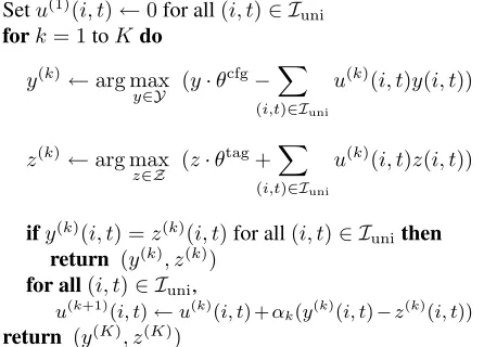
Dual decomposition exploits this idea; it results in the algorithm given in figure 1. The algorithm opti-mizes the combined objective by repeatedly solving the two sub-problems separately—that is, it directly

Setu(1)(i, t)←0for all(i, t)∈ Iuni

fork= 1toKdo

y(k)←arg max

y∈Y (y·θ

cfg₋X

(i,t)∈Iuni

u(k)(i, t)y(i, t))

z(k)←arg max

z∈Z (z·θ

tag₊X

(i,t)∈Iuni

u(k)(i, t)z(i, t))

ify(k)_{(i, t) =z}(k)_{(i, t)for all(i, t)∈ I} unithen

return (y(k)_{, z}(k)₎

for all(i, t)∈ Iuni,

u(k+1)(i, t)←u(k)(i, t) +αk(y(k)(i, t)−z(k)(i, t)) return (y(K), z(K))

Figure 1: The algorithm for integrated parsing and tag-ging. The parametersαk > 0for k = 1. . . K specify

step sizes for each iteration, and are discussed further in the Appendix. The twoarg maxproblems can be solved using dynamic programming.

solves the harder optimization problem using an ex-isting CFG parser and trigram tagger. After each iteration the algorithm adjusts the weights u(i, t); these updates modify the objective functions for the two models, encouraging them to agree on the same POS sequence. In section 6.1 we will show that the variablesu(i, t)are Lagrange multipliers enforcing agreement constraints, and that the algorithm corre-sponds to a (sub)gradient method for optimization of a dual function. The algorithm is easy to imple-ment: all that is required is a decoding algorithm for each of the two models, and simple additive updates to the Lagrange multipliers enforcing agreement be-tween the two models.

4.2 Integrating Two Lexicalized Parsers

Our second example problem is the integration of a phrase-structure parser with a higher-order depen-dency parser. The goal is to add higher-order fea-tures to phrase-structure parsing without greatly in-creasing the complexity of inference.

First, we define an index set for second-order un-labeled projective dependency parsing. The second-order parser considers first-second-order dependencies, as well as grandparent and sibling second-order depen-dencies (e.g., see Carreras (2007)). We assume that

dependen-cies,I0_dep=I_dep∪ I_first, where

Ifirst={(i, j) : i∈ {0. . . n}, j ∈ {1. . . n}, i6=j}

Here (i, j) represents a dependency with head wi and modifierwj(i= 0corresponds to the root sym-bol in the parse). We useD ⊆ {0,1}|Idep0 |_{to denote}

the set of valid projective dependency parses. The second model we use is a lexicalized CFG. Each symbol in the grammar takes the form A(h)

whereA ∈ N is a non-terminal, andh ∈ {1. . . n}

is an index specifying thatwhis the head of the con-stituent. Rule productions take the form hA(a) →

B(b) C(c), i, k, ji whereb ∈ {i . . . k}, c ∈ {(k+ 1). . . j}, and a is equal to b or c, depending on whether A receives its head-word from its left or right child. Each such rule implies a dependency

(a, b) if a = c, or(a, c) if a = b. We takeI_head

to be the index set of all such rules, and I_head0 =

I_head∪ I_firstto be the extended index set. We define

H ⊆ {0,1}|I0

head|_{to be the set of valid parse trees.}

The integrated parsing problem is then to find

(y∗, d∗) = arg max (y,d)∈R

y·θhead+d·θdep (3)

where R = {(y, d) :y∈ H, d∈ D,

y(i, j) =d(i, j)for all (i, j)∈ Ifirst}

This problem has a very similar structure to the problem of integrated parsing and tagging, and we can derive a similar dual decomposition algorithm. The Lagrange multipliers u are a vector in R|Ifirst|

enforcing agreement between dependency assign-ments. The algorithm (omitted for brevity) is identi-cal to the algorithm in figure 1, but withI_uni,Y,Z,

θcfg, andθtagreplaced withIfirst,H,D,θhead, and θdep respectively. The algorithm only requires de-coding algorithms for the two models, together with simple updates to the Lagrange multipliers.

5 Marginal Polytopes and LP Relaxations

We now give formal guarantees for the algorithms in the previous section, showing that they solve LP relaxations of the problems in Eqs. 2 and 3.

To make the connection to linear programming, we first introduce the idea ofmarginal polytopesin section 5.1. In section 5.2, we give a precise state-ment of the LP relaxations that are being solved by the example algorithms, making direct use of marginal polytopes. In section 6 we will prove that the example algorithms solve these LP relaxations.

5.1 Marginal Polytopes

For a finite setY, define the set of all distributions over elements in Y as ∆ = {α ∈ R|Y| : αy ≥

0,P

y∈Yαy = 1}. Eachα ∈ ∆gives a vector of marginals,µ = P

y∈Yαyy, whereµr can be inter-preted as the probability thatyr = 1for ayselected at random from the distributionα.

The set of all possible marginal vectors, known as themarginal polytope, is defined as follows:

M={µ∈Rm:∃α∈∆ such thatµ=

X

y∈Y

αyy}

Mis also frequently referred to as theconvex hullof

Y, written asconv(Y). We use the notationconv(Y)

in the remainder of this paper, instead ofM. For an arbitrary set Y, the marginal polytope

conv(Y) can be complex to describe.6 However, Martin et al. (1990) show that for a very general class of dynamic programming problems, the cor-responding marginal polytope can be expressed as

conv(Y) ={µ∈Rm :Aµ=b, µ≥0} (4)

whereAis ap×mmatrix,bis vector inRp, and the

valuep is linear in the size of a hypergraph repre-sentation of the dynamic program. Note thatAand

bspecify a set ofplinear constraints.

We now give an explicit description of the re-sulting constraints for CFG parsing:7 similar con-straints arise for other dynamic programming algo-rithms for parsing, for example the algoalgo-rithms of Eisner (2000). The exact form of the constraints, and the fact that they are polynomial in number, is not essential for the formal results in this paper. How-ever, a description of the constraints gives valuable intuition for the structure of the marginal polytope.

The constraints are given in figure 2. To develop some intuition, consider the case where the variables

µr are restricted to be binary: hence each binary vector µ specifies a parse tree. The second con-straint in Eq. 5 specifies that exactly one rule must be used at the top of the tree. The set of constraints in Eq. 6 specify that for each production of the form

6_{For any finite setY, conv(Y)can be expressed as{µ ∈}

Rm:Aµ≤b}whereAis a matrix of dimensionp×m, and

b∈Rp(see, e.g., Korte and Vygen (2008), pg. 65). The value forpdepends on the setY, and can be exponential in size.

∀r∈ I0

, µr ≥0 ;

X

X,Y,Z∈N

k=1...(n−1)

µ(X→Y Z,1, k, n) = 1 (5)

∀X∈N,∀(i, j)such that1≤i < j≤nand(i, j)6= (1, n):

X

Y,Z∈N

k=i...(j−1)

µ(X→Y Z, i, k, j) = X

Y,Z∈N

k=1...(i−1)

µ(Y →Z X, k, i−1, j)

+ X

Y,Z∈N

k=(j+1)...n

µ(Y →X Z, i, j, k) (6)

∀Y ∈T, ∀i∈ {1. . . n}: µ(i, Y) =

X

X,Z∈N

k=(i+1)...n

µ(X→Y Z, i, i, k) +X

X,Z∈N

k=1...(i−1)

µ(X →Z Y, k, i−1, i) (7)

Figure 2: The linear constraints defining the marginal polytope for CFG parsing.

hX → Y Z, i, k, ji in a parse tree, there must be exactly one production higher in the tree that gener-ates(X, i, j)as one of its children. The constraints in Eq. 7 enforce consistency between the µ(i, Y)

variables and rule variables higher in the tree. Note that the constraints in Eqs.(5–7) can be written in the formAµ=b,µ≥0, as in Eq. 4.

Under these definitions, we have the following:

Theorem 5.1 Define Y to be the set of all CFG parses, as defined in section 4. Then

conv(Y) ={µ∈_Rm _{:µsatisifies Eqs.(5–7)}}

Proof:This theorem is a special case of Martin et al. (1990), theorem 2.

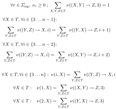
The marginal polytope for tagging,conv(Z), can also be expressed using linear constraints as in Eq. 4; see figure 3. These constraints follow from re-sults for graphical models (Wainwright and Jordan, 2008), or from the Martin et al. (1990) construction. As a final point, the following theorem gives an important property of marginal polytopes, which we will use at several points in this paper:

Theorem 5.2 (Korte and Vygen (2008), page 66.) For any setY ⊆ {0,1}k_{, and for any vectorθ∈}

Rk,

max

y∈Y y·θ=µ∈maxconv(Y)µ·θ (8)

The theorem states that for a linear objective func-tion, maximization over a discrete set Y can be replaced by maximization over the convex hull

∀r∈ I0

tag, νr≥0 ;

X

X,Y,Z∈T

ν((X, Y)→Z,3) = 1

∀X ∈T,∀i∈ {3. . . n−1}:

X

Y,Z∈T

ν((Y, Z)→X, i) = X

Y,Z∈T

ν((Y, X)→Z, i+ 1)

∀X ∈T,∀i∈ {3. . . n−2}:

X

Y,Z∈T

ν((Y, Z)→X, i) = X

Y,Z∈T

ν((X, Y)→Z, i+ 2)

∀X ∈T,∀i∈ {3. . . n}: ν(i, X) = X

Y,Z∈T

ν((Y, Z)→X, i)

∀X∈T : ν(1, X) = X

Y,Z∈T

ν((X, Y)→Z,3)

∀X∈T : ν(2, X) = X

Y,Z∈T

ν((Y, X)→Z,3)

Figure 3: The linear constraints defining the marginal polytope for trigram POS tagging.

conv(Y). The problemmaxµ∈conv(Y)µ·θis a linear

programming problem.

For parsing, this theorem implies that:

1. Weighted CFG parsing can be framed as a linear programming problem, of the formmaxµ∈conv(Y)µ· θ, whereconv(Y)is specified by a polynomial num-ber of linear constraints.

2. Conversely, dynamic programming algorithms such as the CKY algorithm can be considered to be oracles that efficiently solve LPs of the form

maxµ∈conv(Y)µ·θ.

Similar results apply for the POS tagging case.

5.2 Linear Programming Relaxations

We now describe the LP relaxations that are solved by the example algorithms in section 4. We begin with the algorithm in Figure 1.

The original optimization problem was to find

max(y,z)∈Q y·θcfg+z·θtag

(see Eq. 2). By the-orem 5.2, this is equivalent to solving

max (µ,ν)∈conv(Q)

µ·θcfg+ν·θtag

(9)

To formulate our approximation, we first define:

Q0 ={(µ, ν) :µ∈conv(Y), ν ∈conv(Z),

The definition ofQ0is very similar to the definition ofQ (see Eq. 1), the only difference being that Y

and Z are replaced by conv(Y) and conv(Z) re-spectively. Hence any point inQis also inQ0. It fol-lows that any point inconv(Q)is also inQ0_{, because}

Q0 is a convex set defined by linear constraints. The LP relaxation then corresponds to the follow-ing optimization problem:

max (µ,ν)∈Q0

µ·θcfg+ν·θtag (10)

Q0 is defined by linear constraints, making this a linear program. Since Q0 _{is an outer bound on}

conv(Q), i.e.conv(Q)⊆ Q0, we obtain the guaran-tee that the value of Eq. 10 always upper bounds the value of Eq. 9.

In Appendix A we give an example showing that in general Q0 includes points that are not in

conv(Q). These points exist because the agreement between the two parts is now enforced in expecta-tion (µ(i, t) = ν(i, t) for(i, t) ∈ Iuni) rather than

based on actual assignments. This agreement con-straint is weaker since different distributions over assignments can still result in the same first order expectations. Thus, the solution to Eq. 10 may be in Q0 but not in conv(Q). It can be shown that all such solutions will be fractional, making them easy to distinguish fromQ. In many applications of LP relaxations—including the examples discussed in this paper—the relaxation in Eq. 10 turns out to betight, in that the solution is often integral (i.e., it is in Q). In these cases, solving the LP relaxation

exactlysolves the original problem of interest. In the next section we prove that the algorithm in Figure 1 solves the problem in Eq 10. A similar result holds for the algorithm in section 4.2: it solves a relaxation of Eq. 3, whereRis replaced by

R0={(µ, ν) :µ∈conv(H), ν ∈conv(D),

µ(i, j) =ν(i, j)for all (i, j)∈ I_first}

6 Convergence Guarantees

6.1 Lagrangian Relaxation

We now show that the example algorithms solve their respective LP relaxations given in the previ-ous section. We do this by first introducing a gen-eral class of linear programs, together with an op-timization method,Lagrangian relaxation, for solv-ing these LPs. We then show that the algorithms in section 4 are special cases of the general algorithm.

The linear programs we consider take the form

max

x1∈X1,x2∈X2(θ1·x1+θ2·x2) such thatEx1=F x2

The matricesE∈_Rq×m_{andF ∈}

Rq×lspecifyq

lin-ear “agreement” constraints betweenx1 ∈ Rm and x2 ∈Rl. The setsX1,X2are also specified by linear

constraints, X1 = {x1 ∈Rm:Ax1 =b, x1≥0}

andX2 =

x2 ∈Rl:Cx2 =d, x2 ≥0 , hence the

problem is an LP.

Note that if we set X1 = conv(Y), X2 = conv(Z), and defineE andF to specify the agree-ment constraintsµ(i, t) = ν(i, t), then we have the LP relaxation in Eq. 10.

It is natural to apply Lagrangian relaxation in cases where the sub-problemsmaxx1∈X1θ1·x1and

maxx2∈X2θ2·x2 can be efficiently solved by

com-binatorial algorithms for any values of θ1, θ2, but

where the constraintsEx1 =F x2“complicate” the

problem. We introduce Lagrange multipliersu∈_Rq that enforce the latter set of constraints, giving the Lagrangian:

L(u, x1, x2) =θ1·x1+θ2·x2+u·(Ex1−F x2)

The dual objective function is

L(u) = max

x1∈X1,x2∈X2L(u, x1, x2)

and the dual problem is to findmin_u∈RqL(u). Because X1 and X2 are defined by linear

con-straints, by strong duality we have

min

u∈_Rq

L(u) = max

x1∈X1,x2∈X2:Ex1=F x2

(θ1·x1+θ2·x2)

Hence minimizingL(u)will recover the maximum value of the original problem. This leaves open the question of how to recover the LP solution (i.e., the pair (x∗₁, x∗₂) that achieves this maximum); we dis-cuss this point in section 6.2.

The dual L(u) is convex. However, L(u) is not differentiable, so we cannot use gradient-based methods to optimize it. Instead, a standard approach is to use a subgradient method. Subgradients are tan-gent lines that lower bound a function even at points of non-differentiability: formally, a subgradient of a convex functionL:Rn_{→ Rat a pointuis a vector}

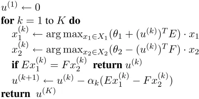
u(1)←0

fork= 1toKdo

x(₁k)←arg maxx1∈X1(θ1+ (u

(k)₎T_E)·x

1

x(₂k)←arg maxx2∈X2(θ2−(u

(k)₎T_F)·x

2

ifEx(₁k)=F x₂(k) returnu(k) u(k+1)←u(k)−αk(Ex(1k)−F x

(k)

2 )

return u(K)

Figure 4: The Lagrangian relaxation algorithm.

By standard results, the subgradient forLat a point

utakes a simple form,gu =Ex∗1−F x∗2, where

x∗₁ = arg max

x1∈X1

(θ1+ (u(k))TE)·x1

x∗₂ = arg max

x2∈X2

(θ2−(u(k))TF)·x2

The beauty of this result is that the values ofx∗₁ and

x∗₂, and by implication the value of the subgradient, can be computed using oracles for the twoarg max

sub-problems.

Subgradient algorithms perform updates that are similar to gradient descent:

u(k+1)←u(k)−αkg(k)

whereg(k)is the subgradient ofLatu(k)andαk>0 is the step size of the update. The complete sub-gradient algorithm is given in figure 4. The follow-ing convergence theorem is well-known (e.g., see page 120 of Korte and Vygen (2008)):

Theorem 6.1 If limk→∞αk = 0andP∞k=1αk =

∞, thenlimk→∞L(u(k)) = minuL(u).

The following proposition is easily verified:

Proposition 6.1 The algorithm in figure 1 is an in-stantiation of the algorithm in figure 4,8 withX1 = conv(Y),X2 = conv(Z), and the matrices E and F defined to be binary matrices specifying the con-straintsµ(i, t) =ν(i, t)for all(i, t)∈ Iuni.

Under an appropriate definition of the step sizesαk, it follows that the algorithm in figure 1 defines a sequence of Lagrange multiplersu(k) minimizing a dual of the LP relaxation in Eq. 10. A similar result holds for the algorithm in section 4.2.

8

with the caveat that it returns(x(₁k), x₂(k))rather thanu(k) .

6.2 Recovering the LP Solution

The previous section described how the method in figure 4 can be used to minimize the dualL(u)of the original linear program. We now turn to the problem of recovering a primal solution (x∗₁, x∗₂) of the LP. The method we propose considers two cases:

(Case 1) If Ex(₁k) = F x(₂k) at any stage during the algorithm, then simply take(x(₁k), x(₂k))to be the primal solution. In this case the pair(x(₁k), x(₂k)) ex-actlysolves the original LP.9If this case arises in the algorithm in figure 1, then the resulting solution is binary (i.e., it is a member ofQ), and the solution exactly solves the original inference problem.

(Case 2) If case 1 does not arise, then a couple of strategies are possible. (This situation could arise in cases where the LP is not tight—i.e., it has a fractional solution—or whereKis not large enough for convergence.) The first is to define the pri-mal solution to be the average of the solutions en-countered during the algorithm: xˆ1 = Pkx

(k)

1 /K,

ˆ

x2 =Pkx

(k)

2 /K. Results from Nedi´c and Ozdaglar

(2009) show that asK → ∞, these averaged solu-tions converge to the optimal primal solution.10 A second strategy (as given in figure 1) is to simply take(x(₁K), x(₂K))as an approximation to the primal solution. This method is a heuristic, but previous work (e.g., Komodakis et al. (2007)) has shown that it is effective in practice; we use it in this paper.

In our experiments we found that in the vast ma-jority of cases, case 1 applies, after a small number of iterations; see the next section for more details.

7 Experiments

7.1 Integrated Phrase-Structure and Dependency Parsing

Our first set of experiments considers the integration of Model 1 of Collins (2003) (a lexicalized phrase-structure parser, from here on referred to as Model

9

We have thatθ1·x(1k)+θ2·x(2k)=L(u (k)

, x(1k), x (k) 2 ) =

L(u(k)_{), where the last equality is becausex}(k) 1 andx

(k) 2 are de-fined by the respectivearg max’s. Thus,(x(1k), x

(k) 2 )andu

(k)

are primal and dual optimal.

Itn. 1 2 3 4 5-10 11-20 20-50 ** Dep 43.5 20.1 10.2 4.9 14.0 5.7 1.4 0.4 POS 58.7 15.4 6.3 3.6 10.3 3.8 0.8 1.1

Table 1: Convergence results for Section 23 of the WSJ Treebank for the dependency parsing and POS experi-ments. Each column gives the percentage of sentences whoseexactsolutions were found in a given range of sub-gradient iterations. ** is the percentage of sentences that did not converge by the iteration limit (K=50).

1),11 and the 2nd order discriminative dependency parser of Koo et al. (2008). The inference problem for a sentencexis to find

y∗ = arg max

y∈Y (f1(y) +γf2(y)) (11)

whereYis the set of all lexicalized phrase-structure trees for the sentencex;f1(y)is the score (log

prob-ability) under Model 1;f2(y)is the score under Koo

et al. (2008) for the dependency structure implied byy; andγ >0is a parameter dictating the relative weight of the two models.12 _{This problem is}

simi-lar to the second example in section 4; a very sim-ilar dual decomposition algorithm to that described in section 4.2 can be derived.

We used the Penn Wall Street Treebank (Marcus et al., 1994) for the experiments, with sections 2-21 for training, section 22 for development, and section 23 for testing. The parameterγ was chosen to opti-mize performance on the development set.

We ran the dual decomposition algorithm with a limit ofK = 50 iterations. The dual decomposi-tion algorithm returns an exact soludecomposi-tion if case 1 oc-curs as defined in section 6.2; we found that of 2416 sentences in section 23, case 1 occurred for 2407 (99.6%) sentences. Table 1 gives statistics showing the number of iterations required for convergence. Over 80% of the examples converge in 5 iterations or fewer; over 90% converge in 10 iterations or fewer.

We compare the accuracy of the dual decomposi-tion approach to two baselines: first, Model 1; and second, a naive integration method that enforces the hard constraint that Model 1 must only consider

de-11

We use a reimplementation that is a slight modification of Collins Model 1, with very similar performance, and which uses the TAG formalism of Carreras et al. (2008).

12

Note that the modelsf1 and f2 were trained separately, using the methods described by Collins (2003) and Koo et al. (2008) respectively.

Precision Recall F1 Dep

Model 1 88.4 87.8 88.1 91.4

Koo08 Baseline 89.9 89.6 89.7 93.3 DD Combination 91.0 90.4 90.7 93.8

Table 2: Performance results for Section 23 of the WSJ Treebank. Model 1: a reimplementation of the genera-tive parser of (Collins, 2002). Koo08 Baseline: Model 1 with a hard restriction to dependencies predicted by the discriminative dependency parser of (Koo et al., 2008). DD Combination: a model that maximizes the joint score of the two parsers. Dep shows the unlabeled dependency accuracy of each system.

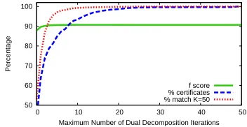
50 60 70 80 90 100

0 10 20 30 40 50

Percentage

Maximum Number of Dual Decomposition Iterations f score % certificates % match K=50

Figure 5: Performance on the parsing task assuming a fixed number of iterationsK. f-score: accuracy of the method. % certificates: percentage of examples for which a certificate of optimality is provided. % match: percent-age of cases where the output from the method is identical to the output when usingK= 50.

pendencies seen in the first-best output from the de-pendency parser. Table 2 shows all three results. The dual decomposition method gives a significant gain in precision and recall over the naive combination method, and boosts the performance of Model 1 to a level that is close to some of the best single-pass parsers on the Penn treebank test set. Dependency accuracy is also improved over the Koo et al. (2008) model, in spite of the relatively low dependency ac-curacy of Model 1 alone.

Figure 5 shows performance of the approach as a function ofK, the maximum number of iterations of dual decomposition. For this experiment, for cases where the method has not converged for k ≤ K, the output from the algorithm is chosen to be the

y(k) fork ≤ K that maximizes the objective func-tion in Eq. 11. The graphs show that values of K

less than 50 produce almost identical performance to

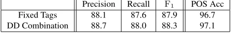
Precision Recall F1 POS Acc

Fixed Tags 88.1 87.6 87.9 96.7

DD Combination 88.7 88.0 88.3 97.1

Table 3: Performance results for Section 23 of the WSJ. Model 1 (Fixed Tags): a baseline parser initialized to the best tag sequence of from the tagger of Toutanova and Manning (2000). DD Combination: a model that maxi-mizes the joint score of parse and tag selection.

7.2 Integrated Phrase-Structure Parsing and Trigram POS tagging

In a second experiment, we used dual decomposi-tion to integrate the Model 1 parser with the Stan-ford max-ent trigram POS tagger (Toutanova and Manning, 2000), using a very similar algorithm to that described in section 4.1. We use the same train-ing/dev/test split as in section 7.1. The two models were again trained separately.

We ran the algorithm with a limit of K = 50 it-erations. Out of 2416 test examples, the algorithm found an exact solution in 98.9% of the cases. Ta-ble 1 gives statistics showing the speed of conver-gence for different examples: over 94% of the exam-ples converge to an exact solution in 10 iterations or fewer. In terms of accuracy, we compare to a base-line approach of using the first-best tag sequence as input to the parser. The dual decomposition ap-proach gives 88.3 F1 measure in recovering parse-tree constituents, compared to 87.9 for the baseline.

8 Conclusions

We have introduced dual-decomposition algorithms for inference in NLP, given formal properties of the algorithms in terms of LP relaxations, and demon-strated their effectiveness on problems that would traditionally be solved using intersections of dy-namic programs (Bar-Hillel et al., 1964). Given the widespread use of dynamic programming in NLP, there should be many applications for the approach. There are several possible extensions of the method we have described. We have focused on cases where two models are being combined; the extension to more than two models is straightfor-ward (e.g., see Komodakis et al. (2007)). This paper has considered approaches for MAP inference; for closely related methods that compute approximate marginals, see Wainwright et al. (2005b).

A Fractional Solutions

We now give an example of a point(µ, ν)∈ Q0_\conv(Q) that demonstrates that the relaxationQ0 _{is strictly larger} thanconv(Q). Fractional points such as this one can arise as solutions of the LP relaxation for worst case instances, preventing us from finding an exact solution.

Recall that the constraints for Q0 _{specify that µ ∈}

conv(Y), ν ∈ conv(Z), and µ(i, t) = ν(i, t) for all

(i, t) ∈ Iuni. Since µ ∈ conv(Y), µ must be a

con-vex combination of1 or more members ofY; a similar property holds forν. The example is as follows. There are two possible parts of speech,AandB, and an addi-tional non-terminal symbolX. The sentence is of length 3, w1 w2 w3. Letν be the convex combination of the

following two tag sequences, each with probability0.5: w1/A w2/A w3/Aandw1/A w2/B w3/B. Letµbe

the convex combination of the following two parses, each with probability0.5:(X(A w1)(X(A w2)(B w3)))and (X(A w1)(X(B w2)(A w3))). It can be verified that µ(i, t) =ν(i, t)for all(i, t), i.e., the marginals for single tags forµandνagree. Thus,(µ, ν)∈ Q0_.

To demonstrate that this fractional point is not in

conv(Q), we give parameter values such that this frtional point is optimal and all integral points (i.e., ac-tual parses) are suboptimal. For the tagging model, set θ(AA→A,3) =θ(AB→B,3) = 0, with all other pa-rameters having a negative value. For the parsing model, setθ(X → A X,1,1,3) = θ(X → A B,2,2,3) =

θ(X →B A,2,2,3) = 0, with all other rule parameters being negative. For this objective, the fractional solution has value0, while all integral points (i.e., all points inQ) have a negative value. By Theorem 5.2, the maximum of any linear objective overconv(Q)is equal to the maxi-mum overQ. Thus,(µ, ν)6∈conv(Q).

B Step Size

We used the following step size in our experiments. First, we initializedα0 to equal 0.5, a relatively large value.

Then we definedαk =α0∗2−ηk, whereηk is the

num-ber of times thatL(u(k0))> L(u(k0−1))fork0 ≤k. This learning rate drops at a rate of1/2t, wheretis the num-ber of times that the dual increases from one iteration to the next. See Koo et al. (2010) for a similar, but less ag-gressive step size used to solve a different task.

References

Y. Bar-Hillel, M. Perles, and E. Shamir. 1964. On formal properties of simple phrase structure grammars. In

Language and Information: Selected Essays on their Theory and Application, pages 116–150.

X. Carreras, M. Collins, and T. Koo. 2008. TAG, dy-namic programming, and the perceptron for efficient, feature-rich parsing. InProc CONLL, pages 9–16. X. Carreras. 2007. Experiments with a higher-order

projective dependency parser. InProc. CoNLL, pages 957–961.

M. Collins. 2002. Discriminative training methods for hidden markov models: Theory and experiments with perceptron algorithms. InProc. EMNLP, page 8. M. Collins. 2003. Head-driven statistical models for

nat-ural language parsing. In Computational linguistics, volume 29, pages 589–637.

G.B. Dantzig and P. Wolfe. 1960. Decomposition princi-ple for linear programs. InOperations research, vol-ume 8, pages 101–111.

J. Duchi, D. Tarlow, G. Elidan, and D. Koller. 2007. Using combinatorial optimization within max-product belief propagation. InNIPS, volume 19.

J. Eisner. 2000. Bilexical grammars and their cubic-time parsing algorithms. InAdvances in Probabilistic and Other Parsing Technologies, pages 29–62.

A. Globerson and T. Jaakkola. 2007. Fixing max-product: Convergent message passing algorithms for MAP LP-relaxations. InNIPS, volume 21.

N. Komodakis, N. Paragios, and G. Tziritas. 2007. MRF optimization via dual decomposition: Message-passing revisited. In International Conference on Computer Vision.

T. Koo, X. Carreras, and M. Collins. 2008. Simple semi-supervised dependency parsing. InProc. ACL/HLT. T. Koo, A.M. Rush, M. Collins, T. Jaakkola, and D.

Son-tag. 2010. Dual Decomposition for Parsing with Non-Projective Head Automata. InProc. EMNLP, pages 63–70.

B.H. Korte and J. Vygen. 2008. Combinatorial optimiza-tion: theory and algorithms. Springer Verlag.

M.P. Marcus, B. Santorini, and M.A. Marcinkiewicz. 1994. Building a large annotated corpus of English: The Penn Treebank. InComputational linguistics, vol-ume 19, pages 313–330.

R.K. Martin, R.L. Rardin, and B.A. Campbell. 1990. Polyhedral characterization of discrete dynamic pro-gramming. Operations research, 38(1):127–138. A.F.T. Martins, N.A. Smith, and E.P. Xing. 2009.

Con-cise integer linear programming formulations for de-pendency parsing. InProc. ACL.

R. McDonald, F. Pereira, K. Ribarov, and J. Hajic. 2005. Non-projective dependency parsing using spanning tree algorithms. In Proc. HLT/EMNLP, pages 523– 530.

Angelia Nedi´c and Asuman Ozdaglar. 2009. Approxi-mate primal solutions and rate analysis for dual sub-gradient methods. SIAM Journal on Optimization, 19(4):1757–1780.

B. Pang and L. Lee. 2004. A sentimental education: Sentiment analysis using subjectivity summarization based on minimum cuts. InProc. ACL.

S. Riedel and J. Clarke. 2006. Incremental integer linear programming for non-projective dependency parsing. InProc. EMNLP, pages 129–137.

D. Roth and W. Yih. 2005. Integer linear program-ming inference for conditional random fields. InProc. ICML, pages 737–744.

Hanif D. Sherali and Warren P. Adams. 1994. A hi-erarchy of relaxations and convex hull characteriza-tions for mixed-integer zero–one programming prob-lems. Discrete Applied Mathematics, 52(1):83 – 106. D.A. Smith and J. Eisner. 2008. Dependency parsing by

belief propagation. InProc. EMNLP, pages 145–156. D. Sontag, T. Meltzer, A. Globerson, T. Jaakkola, and

Y. Weiss. 2008. Tightening LP relaxations for MAP using message passing. InProc. UAI.

B. Taskar, D. Klein, M. Collins, D. Koller, and C. Man-ning. 2004. Max-margin parsing. InProc. EMNLP, pages 1–8.

K. Toutanova and C.D. Manning. 2000. Enriching the knowledge sources used in a maximum entropy part-of-speech tagger. InProc. EMNLP, pages 63–70. M. Wainwright and M. I. Jordan. 2008. Graphical

Mod-els, Exponential Families, and Variational Inference. Now Publishers Inc., Hanover, MA, USA.

M. Wainwright, T. Jaakkola, and A. Willsky. 2005a. MAP estimation via agreement on trees: message-passing and linear programming. In IEEE Transac-tions on Information Theory, volume 51, pages 3697– 3717.

M. Wainwright, T. Jaakkola, and A. Willsky. 2005b. A new class of upper bounds on the log partition func-tion. In IEEE Transactions on Information Theory, volume 51, pages 2313–2335.