COMPOSITIONAL REASONING FOR EXPLICIT RESOURCE MANAGEMENT IN CHANNEL-BASED CONCURRENCY∗
ADRIAN FRANCALANZAa, EDSKO DEVRIESb, AND MATTHEW HENNESSYc
aICT, University of Malta
e-mail address: [email protected]
bWell-Typed LLP, UK
e-mail address: [email protected]
cTrinity College Dublin, Ireland
e-mail address: [email protected]
Abstract. We define aπ-calculus variant with a costed semantics where channels are treated as
re-sources that must explicitly be allocated before they are used and can be deallocated when no longer required. We use a substructural type system tracking permission transfer to construct coinductive proof techniques for comparing behaviour and resource usage efficiency of concurrent processes. We establish full abstraction results between our coinductive definitions and a contextual behavioural preorder describing a notion of process efficiencywrt. its management of resources. We also jus-tify these definitions and respective proof techniques through numerous examples and a case study comparing two concurrent implementations of an extensible buffer.
1. Introduction
We investigate the behaviour and space efficiency of concurrent programs with explicit resource-management. In particular, our study focuses on channel-passing concurrent programs: we define a
π-calculus variant, called Rπ, where the only resources available are channels; these channels must explicitly be allocated before they can be used, and can be deallocated when no longer required. As part of the operational model of the language, channel allocation and deallocation have costs associated with them, reflecting the respective resource usage.
Explicit resource management is typically desirable in settings where resources are scarce. Re-source management programming constructs such as explicit deallocation provide fine-grained con-trol over how these resources are used and recycled. By comparison, in automated mechanisms such as garbage collection, unused resources (in this case, memory) tend to remain longer in an unreclaimed state [27, 28]. Explicit resource management constructs such as memory deallocation also carry advantages over automated mechanisms such as garbage collection techniques when it
2012 ACM CCS: [Theory of computation]: Models of Computation—Concurrency—Process Calculi. Key words and phrases: π-calculus, concurrency, memory management, coinductive reasoning. ∗An extended abstract of a preliminary version of the paper has appeared in [11].
cSupported by SFI project SFI 06 IN.1 1898.
LOGICAL METHODS
lIN COMPUTER SCIENCE DOI:10.2168/LMCS-10(2:15)2014
c
A. Francalanza, E. DeVries, and M. Hennessy
CC
comes to interactive and real-time programs [10, 27, 28]. In particular, garbage collection tech-niques require additional computation to determine otherwise explicit information as to which parts of the memory to reclaim and at what stage of the computation; the associated overheads may lead to uneven performance and intolerable pause periods where the system becomes unresponsive [10]. In the case of channel-passing concurrency with explicit memory-management, the analysis of the relative behaviour and efficiency of programs is non-trivial for a number of reasons. Explicit memory-management introduces the risk of either premature or multiple deallocation of resources along separate threads of execution; these are more difficult to detect than in single-threaded pro-grams and potentially result in problems such as wild pointers or corrupted heaps which may, in turn, lead to unpredictable, even catastrophic, behaviour [27, 28]. It also increases the possibility of memory leaks, which are often not noticeable in short-running, terminating programs but subtly eat up resources over the course of long-running programs. In a concurrent settings such as ours, complications relating to the assessment and comparison of resource consumption is further com-pounded by the fact that the runtime execution of channel-passing concurrent programs can have multiple interleavings, is sometimes non-deterministic and often non-terminating.
1.1. Scenario: Consider a setting with two servers, S1and S2, which repeatedly listen for service
requests on channelssrv1andsrv2, respectively. Requests send a return channel onsrv1orsrv2 which is then used by the servers to service the requests and send back answers, v1 and v2. A
possible implementation for these servers is given in (1.1) below, whererecw.P denotes a process P recursing at w, c?x.P denotes a process inputting on channelcsome value that is bound to the variable x in the continuation P, andc!v.P outputs a value v on channelcand continues as P:
Si ,recw.srvi?x. x!vi.w for i∈ {1,2} (1.1)
Clients that need to request service from both servers, so as to report back the outcome of both server interactions on some channel,ret, can be programmed in a variety of ways:
C0 ,recw.allocx1.allocx2.srv1!x1.x1?y.srv2!x2.x2?z.ret!(y,z).w
C1 ,recw.allocx.srv1!x.x?y.srv2!x.x?z.ret!(y,z).w
C2 ,recw.allocx.srv1!x.x?y.srv2!x.x?z.freex.ret!(y,z).w
(1.2)
C0 corresponds to an idiomaticπ-calculus client. In order to ensure that it is the sole recipient of
the service requests, it creates two new return channels to communicate with S1 and S2 onsrv1
and srv2, using the command allocx.P; this command allocates a new channel cand binds it
to the variable x in the continuation P. Allocating a new channel for each service request ensures that the return channel used between the client and server is private for the duration of the service, preventing interferences from other parties executing in parallel.
One important difference between the computational model considered in this paper and that of the standardπ-calculus is that channel allocation is an expensive operationi.e., it incurs an additional (spatial) cost compared to the other operations. Client C1 attempts to address the inefficiencies of
C0 by allocating only one additional new channel, and reusing this channel for both interactions
with the servers. Intuitively, this channel reuse is valid, i.e., it preserves the client-server behaviour C0 had with servers S1 and S2, because the server implementations above use the received
return-channels only once. This single channel usage guarantees that return return-channels remain private during the duration of the service, despite the reuse from client C1.
Client C2 attempts to be more efficient still. More precisely, since our computational model
channels that are not disposed of, even though these channels are never used again in subsequent it-erations. By contrast, C2deallocates unused channels at the end of each iteration using the construct
free c.P.
In this work we develop a formal framework for comparing the behaviour of concurrent pro-cesses that explicitly allocate and deallocate channels. For instance, propro-cesses consisting of the servers S1 and S2 together with any of the clients C0, C1 or C2 should be related, on the basis
that they exhibit the same behaviour. In addition, we would like to order these systems, based on their relative efficiencieswrt. the (channel) resources used. We note that there are various, at times contrasting, notions of efficiency that one may consider. For instance, one notion may consider acquiring memory for long periods to be less efficient than repeatedly allocating and deallocating memory; another notion of efficiency could instead focus on minimising the allocation and deallo-cation operations used, as these as considerably more expensive than other operations. In this work, we mainly focus on a notion of efficiency that accounts for the relative memory allocations required to carry out the necessary computations. Thus, we would intuitively like to develop a framework yielding the following preorder, where⊏∼reads ”more efficient than”:
S1kS2 kC2 ⊏∼ S1kS2 kC1 ⊏∼ S1kS2kC0 (1.3)
A pleasing property of this preorder would be compositionality, which implies that orderings are preserved under larger contexts,i.e., for all (valid) contextsC[−], P⊏∼Q impliesC[P]⊏∼C[Q].
Du-ally, compositionality would also improve the scalability of our formal framework since, to show that C[P]⊏∼C[Q] (for some context C[−]), it suffices to obtain P⊏∼Q. For instance, in the case of
(1.3), compositionality would allow us to factor out the common code,i.e., the servers S1and S2as
the context S1kS2k[−], and focus on showing that
C2⊏∼C1⊏∼C0 (1.4)
1.2. Main Challenges: The details are however far from straightforward. To begin with, we need to assess relative program cost over potentially infinite computations. Thus, rudimentary aggregate measures such as adding up the total computation cost of processes and comparing this total at the end of the computation is insufficient for system comparisons such as (1.3). In such cases, a preliminary attempt at a solution would be to compare the relative cost for every server interaction (action): in the sense of [4], the preorder would then ensure that every costed interaction by the inefficient clients must be matched by a corresponding cheaper interaction by the more efficient client (and, dually, costed interactions by the efficient client must be matched by interactions from the inefficient client that are as costly or more).
C3,recw.allocx1.allocx2. srv1!x1.x1?y. srv2!x2.x2?z. freex1.freex2.ret!(y,z).w (1.5)
There are however problems with this approach. Consider, for instance, C3defined in (1.5). Even
though this client allocates two channels for every iteration of server interactions, it does not exhibit any memory leaks since it deallocates them both at the end of the iteration. It may therefore be sensible for our preorder to equate C3with client C2of (1.2) by having C2 ⊏∼C3as well as C3⊏∼C2.
However showing C3 ⊏∼ C2 would not be possible using the preliminary strategy discussed above,
since, C3must engage in more expensive computation (allocating two channels as opposed to 1) by
the time the interaction with the first server is carried out.
Worse still, an analysis strategy akin to [4] would not be applicable for a comparison involving the clients C1 and C3. In spite of the fact that over the course of its entire computation C3requires
interaction with the first server on channelsrv1since, at that stage, it has allocated two new channels as opposed to one. However, C1 becomes less efficient for the remainder of the iteration since it
never deallocates the channel it allocates whereas C3deallocates both channels. To summarise, for
comparisons C3 ⊏∼ C2 and C3 ⊏∼ C1, we need our analysis to allow a process to be temporarily
inefficient as long as it can recover later on.
In this paper, we use a costed semantics to define an efficiency preorder to reason about the relative cost of processes over potentially infinite computation, based on earlier work by [30, 34]. In particular, we adapt the concept of cost amortisation to our setting, used by our preorders to compare processes that are eventually more efficient than others over the course of their entire computation, but are temporarily less efficient at certain stages of the computation.
Issues concerning cost assessment are however not the only obstacles tackled in this work; there are also complications associated with the compositionality aspects of our proposed framework. More precisely, we want to limit our analysis to safe contexts,i.e., contexts that use resources in a sensible way,e.g., not deallocating channels while they are still in use. In addition, we also want to consider behaviourwrt. a subset of the possible safe contexts. For instance, our clients from (1.2) only exhibit the same behaviour wrt. servers that (i) accept (any number of) requests on channels srv1andsrv2containing a return channel, which then (ii) use this channel at most once to return
the requested answer. We can characterise the interface between the servers and the clients using fairly standard channel type descriptions adapted from [31] in (1.6), where [T]ω
describes a channel than can be used any number of times (i.e., the channel-type attributeω) to communicate values of
type T, whereas [T]1denotes an affine channel (i.e., a channel type with attribute 1) that can be used at most once to communicate values of type T:
srv1 : [[T1]1]ω
, srv2 : [[T2]1]ω
(1.6)
In the style of [45, 21], we could then use this interface to abstract away from the actual server implementations described in (1.1) and state that,wrt. contexts that observe the channel mappings of (1.6), client C2is more efficient than C1which is, in turn, more efficient than C0. These can be
expressed as:
srv1: [[T1]1]ω
,srv2 : [[T2]1]ω
|= C2⊏∼C1 (1.7)
srv1: [[T1]1]ω
,srv2 : [[T2]1]ω
|= C1⊏∼C0 (1.8)
Unfortunately, the machinery of [45, 21] cannot be easily extended to our costed analysis be-cause of two main reasons. First, in order to limit our analysis to safe computation, we would need to show that clients C0, C1and C2adhere to the channel usage stipulated by the type associations
in (1.6). However, the channel reuse in C1 and C2 (an essential feature to attain space efficiency)
requires our analysis to associate potentially different types (i.e., [T1]1 and [T2]1) to the same
re-turn channel; this channel reuse at different types amounts to a form of strong update, a degree of flexibility not supported by [45, 21].
Second, the equivalence reasoning mechanisms used in [45, 21] would be substantially limiting for processes with channel reuse. More specifically, consider the slightly tweaked client implemen-tation of C2below:
C′2,recw.allocx.srv1!x k x?y.(srv2!x k x?z.freex.c!(y,z).X)
(1.9)
The only difference between the client in (1.9) and the original one in (1.2) is that C2 sequences
use that resource have been used up; this feature is essential to statically reason about a number of basic design patterns for reuse. For such type settings, it turns out that the client implementations C2
and C′2 exhibit the same behaviour because the return channel used by both clients for both server interactions is private,i.e., unknown to the respective servers; as a result, the servers cannot answer the service on that channel before it is receives it on either srv1 orsrv2.1 Through scope extru-sion, theories such as [45, 21] can reason adequately about the first server interaction, and relate
. . .srv1!x.x?y. . .of C2 with. . .srv1!x k x?y.. . .of C2. However, they have no mechanism for tracking channel locality post scope extrusion, thereby recovering the information that the return channel becomes private again to the client after the first server interaction (since the servers use up the permission to use the return channel once they reply on it). This prohibits [45, 21] from determining that the second server interaction is just an instance of the first server interaction, thus failing to relate these two implementations.
In [12] we developed a substructural type system based around a type attribute describing chan-nel uniqueness, and this was used to statically ensure safe computations for Rπ. In this work, we weave this type information into our framework, imbuing it with an operational permission-semantics to reason compositionally about the costed behaviour of (safe) processes. More specif-ically, in (1.2), when C2 allocates channel x, no other process knows about x: from a typing
per-spective, but also operationally, x is unique to C2. Client C2then sends x onsrv1at an affine type,
which (by definition) limits the server to use x at most once. At this point, from an operational perspective, x is to C2, the entity previously “owning” it, unique-after-1 (communication) use. This
means that after one communication step on x, (the derivative of) C2recognises that all the other
processes apart from it must have used up the single affine permission for x, and hence x becomes once again unique to C2. This also means that C2can safely reuse x, possibly at a different object
type (strong update), or else safely deallocate it.
The concept of affinity is well-known in the process calculus community. By contrast, unique-ness (and its duality to affinity) is used far less. In a compositional framework, uniqueness can be used to record the guarantee at one end of a channel corresponding to the restriction associated with affine channel usage at the other; an operational semantics can be defined, tracking the permis-sion transfer of affine permissions back and forth between processes as a result of communication, addressing the aforementioned complications associated with idioms such as channel reuse. We employ such an operational (costed) semantics to define our efficiency preorders for concurrent pro-cesses with explicit resource management, based on the notion of amortised cost discussed above.
1.3. Paper Structure: Section 2 introduces our language with constructs for explicit memory man-agement and defines a costed semantics for it. We illustrate issues relating to resource usage in this language through a case study in Section 3, discussing different implementations for an unbounded buffer. Section 4 develops a labelled-transition system for our language that takes into consideration some representation of the observer and the permissions that are exchanged between the program and the observer; it is a typed transition system similar to [38, 21, 19], nuanced to the resource-focussed type system of [12]. Based on this transition system, the section also defines a coinductive cost-based preorder and proves a number of properties about it. Section 5 justifies the cost-based preorder by relating it with a behavioural contextual preorder defined in terms of the reduction se-mantics of Section 2. Section 6 applies the theory of Section 4 to reason about the efficiency of the unbounded buffer implementations of Section 3. Finally, Section 7 surveys related work and Section 8 concludes.
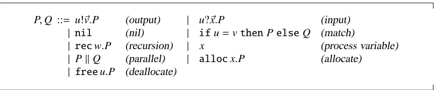
P,Q ::= u!~v.P (output) | u?~x.P (input)
| nil (nil) | ifu=vthenPelseQ (match)
| recw.P (recursion) | x (process variable)
| PkQ (parallel) | allocx.P (allocate)
[image:6.612.91.527.111.201.2]| freeu.P (deallocate)
Figure 1: RπSyntax
2. TheLanguage
Figure 1 shows the syntax for our language, the resource π-calculus, or Rπfor short. It has the standard π-calculus constructs with the exception of scoping, which is replaced with primitives for explicit channel allocation, allocx.P, and deallocation, freex.P. The syntax assumes two separate denumerable sets of channel names c,d ∈ Chan, and variables x,y,z,w ∈ Var, and lets identifiers u,v range over both sets, Chan∪Var. The input construct, c?x.P, recursion construct, recw.P, and channel allocation construct,allocx.P, are binders whereby free occurrences of the variables x and w in P are bound. As opposed to more standard versions of theπ-calculus, we do not use name scoping to bind and bookkeep the visibility of names; we shall however use alternative mechanisms to track name knowledge and usage in subsequent development.
Rπprocesses run in a resource environment, ranged over by M,N, representing predicates over channel names stating whether a channel is allocated or not. We find it convenient to denote such functions as a list of channels representing the set channels that are allocated, e.g., the list c,d de-notes the set{c,d}, representing the resource environment returning true for channels c and d and false otherwise - in this representation, the order of the channels in the list is unimportant, but dupli-cate channels are disallowed; as shorthand, we also write M,c to denote M∪ {c}whenever c<M. In this paper we consider only resource environments with an infinite number of deallocated channels, i.e., M is a total function. Models with finite resources can be easily accommodated by making M partial; this also would entail a slight change in the semantics of the allocation construct, which could either block or fail whenever there are no deallocated resources left. Although interesting in its own right, we focus on settings with infinite resources as it lends itself better to the analysis of resource efficiency that follows.
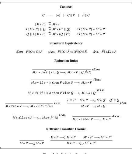
We refer to the pair M⊲P, consisting of a resource environment M and a closed process2P as a system; note that not all free names in P need to be allocatedi.e., present in M: intuitively, any name c used by P and c < M represents a dangling pointer. Contexts consist of parallel composition of processes; they are however defined over systems, through the grammar and the respective definition at the top of Figure 2. The reduction relation is defined as the least contextual relation over systems satisfying the rules in Figure 2. More specifically our reduction relation leaves the following rule implicit:
M⊲P −→k M⊲Q
rCtx C[M⊲P] −→k C[M⊲Q]
2A closed process has no free variables. Note that the absence of name bindersi.e., no name scoping, means that all
Contexts
C ::= [−] | C kP | Pk C
[M⊲P] def= M⊲P
C[M⊲P] k Q def= M′⊲(P′ kQ) ifC[M⊲P]= M′⊲P′ Q k C[M⊲P] def= M′⊲(QkP′) ifC[M⊲P]= M′⊲P′
Structural Equivalence
sCom PkQ≡QkP sAss Pk(QkR)≡(PkQ)kR sNil Pknil≡P
Reduction Rules
rCom M,c⊲c!d~.Pkc?~x.Q−→0 M,c⊲PkQ{d~/~x}
rThen M,c⊲ifc=cthenPelseQ−→0 M,c⊲P
rElse M,c,d⊲ifc=dthenPelseQ−→0 M,c,d⊲Q
rRec M⊲recw.P−→0 M⊲P{recw.P/w}
P≡ P′ M⊲P′−→k M⊲Q′ Q′≡Q
rStr M⊲P−→k M⊲Q
rAll
M⊲allocx.P−→+1 M,c⊲P{c/x} rFree
M,c⊲freec.P−→−1 M⊲P
Reflexive Transitive Closure
M⊲P−→∗0 M⊲P
[image:7.612.89.523.107.610.2]M⊲P−→∗k M′⊲P′ M′⊲P′−→l M′′⊲P′′ M⊲P−→∗k+l M′′⊲P′′
Figure 2: RπReduction Semantics
Rule (rStr) extends reductions to structurally equivalent processes, P ≡ Q,i.e., processes that are identified up to superfluousnilprocesses, and commutativity/associativity of parallel composition (see the structural equivalence rules Figure 2).
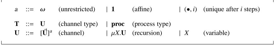
a ::= ω (unrestricted) | 1 (affine) | (•,i) (unique after i steps)
T ::= U (channel type) | proc (process type)
[image:8.612.88.528.116.189.2]U ::= [U]~ a (channel) | µX.U (recursion) | X (variable)
Figure 3: Type Attributes and Types
substitutes it for the bound variable of the allocation construct.3 Deallocation (rFree) changes the states of a channel from allocated to deallocated, making it available for future allocations. The rules are annotated with a cost reflecting resource usage; allocation has a cost of+1, deallocation has a (negative) cost of−1 while the other reductions carry no cost,i.e., 0. Figure 2 also shows the natural definition of the reflexive transitive closure of the costed reduction relation. In what follows, we use k,l∈Zas integer metavariables to range over costs.
Example 2.1. The following reduction sequence illustrates potential unwanted behaviour resulting
from resource mismanagement:
M,c⊲freec.(c!1kc?x.P) k allocy.(y!42ky?z.Q) −→−1 (2.1) M ⊲c!1kc?x.P k allocy.(x!42kx?z.Q) −→+1 (2.2)
M,c⊲c!1kc?x.P k c!42kc?z.Q (2.3)
Intuitively, allocation should yield “fresh” channelsi.e., channels that are not in use by any active process. This assumption is used by the right process in system (2.1), allocy.(y!42 k y?z.Q),
to carry out a local communication, sending the value42 on some local channel y that no other
process is using. However, the premature deallocation of the channel c by the left process in (2.1), freec.(c!1 k c?x.P), allows channel c to be reallocated by the right process in the subsequent reduction, (2.2). This may then lead to unintended behaviour since we may end up with interferences
when communicating on c in the residuals of the left and right processes, (2.3).4
In [12] we defined a type system that precludes unwanted behaviour such as in Example 2.1. The type syntax is shown in Figure 3. The main type entities are channel types, denoted as [U]~ a, where type attributes a range over
• 1, for affine, imposing a restriction/obligation on usage;
• (•,i), for unique-after-i usages (i∈N), providing guarantees on usage;
• ω, for unrestricted channel usage without restrictions or guarantees.
Uniqueness typing can be seen as dual to affine typing [18], and in [12] we make use of this duality to keep track of uniqueness across channel-passing parallel processes: an attribute (•,i) typing an endpoint of a channel c accounts for (at most) i instances of affine attributes typing endpoints of that same channel.
A channel type [U]~ a also describes the type of the values that can be communicated on that channel, U, which denotes a list of types U~ 1, . . . ,Un for n ∈ Nat; when n = 0, the type list is an 3The expected side-condition c<M is implicit in the notation (M,c) used in the system M,c⊲P{c/x}to which it
reduces, since c cannot be present in M for M,c to be valid.
4Operationally, we do not describe errors that may result from attempted communications on deallocated channels
empty list and we simply write []a. Note the difference between [U]~ 1,i.e., a channel with an affine
usage restriction, and [U]~ (•,1),i.e., a channel with a unique-after-1 usage guarantee. We denote fully unique channels as [U]~ •in lieu of [U]~ (•,0).
The type syntax also assumes a denumerable set of type variables X,Y, bound by the recursive type construct µX.U. In what follows, we restrict our attention to closed, contractive types, where
every type variable is bound and appears within a channel constructor [−]a; this ensures that chan-nel types such asµX.X are avoided. We assume an equi-recursive interpretation for our recursive types [36] (seetEqin Figure 4), characterised as the least type-congruence satisfying rule eRecin Figure 4.
Γ⊢P dom(Γ)⊆M Γis consistent
tSys
Γ⊢M⊲P
The rules for typing processes are given in Figure 4 and take the usual shape Γ ⊢ P stating that process P is well-typed with respect to the environmentΓ, a list of pairs of identiers and types. Systems are typed according to (tSys) above: a system M⊲P is well-typed underΓif P is well-typed wrt.Γ,Γ⊢P, andΓonly contains assumptions for channels that have been allocated,dom(Γ)⊆ M. This restricts channel usage in P to allocated channels and is key for ensuring safety.
In [12], typing environments are multisets of pairs of identifiers and types; we do not require them to be partial functions. However, the (top-level) typing rule for systems (tSys) requires that the typing environment is consistent. A typing environment is consistent if whenever it contains multiple assumptions about a channel, then these assumptions can be derived from a single assump-tion using the structural rules of the type system (see the structural ruletConand the splitting rule pUnqin Figure 4).
Definition 2.2 (Consistency). A typing environmentΓis consistent if there is a partial mapΓ′such thatΓ′≺Γ.
The environment structural rules,Γ1 ≺ Γ2, defined in Figure 4, govern the way type environ-ments are syntactically manipulated. For instance, rulestConandtJoinstate that type assumptions for the same identifier can be split or joined according to the type splitting relation T = T1◦T2,
also defined in Figure 4: apart from standard splitting of unrestricted channels,pUnr, and process types,pProc, we note that a unique-after-i channel may be split into a unique-after-(i+1) channel and an affine channel; we also note that affine channels are never split. The environment structural rules also allow for weakening, tWeak, equi-recursive manipulation of types, tEqand eRec, and subtyping,tSub; the latter rule is defined in terms of the subtyping relation also stated in Figure 4 (bottom) where, for instance, an unrestricted channel can be used instead of an affine channel (that can be used at most once). The key novel structural rule is howevertRev, which allows us to change (revise) the object type of a channel whenever we are guaranteed that the type assumption for that identifier is unique. These rules are recalled from [12] and the reader is encouraged to consult that document for more details.
The consistency condition of Definition 2.2 ensures that there is no mismatch in the duality between the guarantees of unique types and the restrictions of affine types, which allows sound compositional type-checking by our type system. For instance, consistency rules out environments such as
c : [U]•,c : [U]1 (2.4)
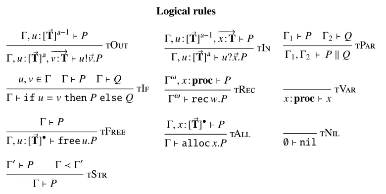
Logical rules
Γ,u : [~T]a−1⊢P
tOut
Γ,u : [T]~ a,−−→v : T⊢u!~v.P
Γ,u : [T]~ a−1,−x : T−−→⊢P tIn
Γ,u : [T]~ a⊢u?~x.P
Γ1 ⊢P Γ2⊢Q
tPar
Γ1,Γ2 ⊢ PkQ u,v∈Γ Γ⊢P Γ⊢Q
tIf
Γ⊢ifu=vthenPelseQ
Γω
,x : proc⊢P tRec
Γω
⊢recw.P
tVar x : proc⊢x
Γ⊢P
tFree
Γ,u : [T]~ •⊢freeu.P
Γ,x : [T]~ •⊢P tAll
Γ⊢allocx.P
tNil ∅ ⊢nil
Γ′⊢P Γ≺Γ′
tStr
Γ⊢P
whereΓω
can only contain unrestricted assumptions and all bound variables are fresh.
Structural rules (≺) is the least reflexive transitive relation satisfying
T=T1◦T2
tCon
Γ,u : T≺Γ,u : T1,u : T2
T=T1◦T2
tJoin
Γ,u : T1,u : T2≺Γ,u : T
T1∼T2
tEq
Γ,u : T1≺Γ,u : T2
tWeak
Γ,u : T≺Γ
T1 ≺sT2
tSub
Γ,u : T1 ≺Γ,u : T2
tRev
Γ,u : [T~1]•≺Γ,u : [T~2]•
Equi-Recursion Counting channel usage
eRec
µX.U∼U{µX.U/X} c : [T]~
a−1def=
ε (empty list) if a=1
c : [T]~ ω
if a=ω
c : [T]~ (•,i) if a=(•,i+1)
Type splitting
pUnr [T]~ ω
=[~T]ω
◦[T]~ ω pProc
proc=proc◦proc [~T](•,i) =[T]~ 1◦[T]~ (•,i+1) pUnq Subtyping
sIndx
(•,i)≺s(•,i+1) (•,i)≺sωsUnq
sAff ω≺s1
a1≺sa2
[image:10.612.118.508.118.314.2]sTyp [T]~ a1 ≺s[~T]a2
For similar reasons, consistency also rules out environments such as
c : [U]•,c : [U]ω
(2.5)
However, it does not rule out environments such as (2.6) even though the guarantee provided by c : [U](•,2) is too conservative: it states that channel c will become unique after two uses but, in actual fact, it becomes unique after one use since the (top-level) environment contains only one other affine type assumption, c : [U]1, that other processes can be typed at.
c : [U](•,2),c : [U]1 (2.6)
A less conservative uniqueness typing guarantee would therefore be c : [U](•,1) as shown in (2.7) below; this environment constitutes another case of a consistent environment allowed by Defini-tion 2.2.
c : [U](•,1),c : [U]1 (2.7)
[image:11.612.138.512.355.433.2]The type system is substructural, implying that typing assumptions can be used only once during typechecking [37]. This is clearly manifested in the output and input rules,tOutandtInin Figure 4. In fact, using the operation c : [~T]a−1(see5Figure 4), rule tOutcollapses three different possibilities for typing output processes, which could alternatively have been expressed as the three separate typing rules in (2.8).
Γ⊢P
tOutA
Γ,u : [~T]1,−−→v : T ⊢ u!~v.P
Γ,u : [T]~ ω ⊢P
tOutW
Γ, u : [T]~ ω
, −−→v : T ⊢ u!~v.P
Γ,u : [~T](•,i) ⊢P
tOutU
Γ, u : [T]~ (•,i+1), −−→v : T ⊢ u!~v.P
(2.8)
RuletOutA states that an output of values~v on channel u is allowed if the type environment has an affine channel-type assumption for that channel, u : [T]~ 1, and the corresponding type assumptions for the values communicated, −−→v : T, match the object type of the affine channel-type assumption,
~
T; in the rule premise, the continuation P must also be typed wrt. the remaining assumptions in
the environment, without the assumptions consumed by the conclusion. Rule tOutW is similar,
but permits outputs on u for environments with an unrestricted channel-type assumption for that channel, u : [~T]ω
. The continuation P is typechecked wrt. the remaining assumptions and a new
assumption, u : [T]~ ω
; this assumption is identical to the one consumed in the conclusion, so as to model the fact that uses of channel u are unrestricted. Rule tOutU is again similar, but it allows outputs on channel u for a “unique after i+1” channel-type assumption; in the premise of the rule, P is typecheckedwrt. the remaining assumptions and a new assumption u : [T]~ (•,i), where u is now unique after i uses. Analogously, the input rule,tIn, also encodes three input cases (listed below):
Γ,−x : T−−→⊢P
tInO
Γ,u : [T]~ 1 ⊢u?~x.P
Γ,u : [T]~ ω
,−x : T−−→⊢P tInW
Γ,u : [T]~ ω
⊢u?~x.P
Γ,u : [T]~ (•,i),−x : T−−→⊢P tInU
Γ,u : [~T](•,i+1)⊢u?~x.P
(2.9)
5This operation on type assumptions, c : [T]~ a−1, defined in Figure 4, describes the cases where, when using an affine
type assumption to typecheck a process, the continuation of the process in the rule premise is typed without that assump-tion (the operaassump-tion returns no type assumpassump-tion), whereas when using an unrestricted or unique-after-i assumpassump-tions, the premise judgement usewrt. (new) unrestricted and unique-after-(i−1) assumptions, respectively. Note that the operation
Parallel composition (tPar) enforces the substructural treatment of type assumptions, by ensuring that type assumptions are used by either the left process or the right, but not by both. However, some type assumption can be split using contraction,i.e., rules (tStr) and (tCon). For example, an assumption c : [T]~ (•,i)can be split as c : [T]~ 1and c : [T]~ (•,i+1)—see (pUnq).
The rest of the rules in Figure 4 are fairly straightforward. Even though these typing rules do not requireΓto be consistent, the consistency requirement at the top level typing judgement (tSys) ensures that whenever a process is typedwrt. a unique assumption for a channel, [~T]•, no other process has access to that channel. It can therefore safely deallocate it (tFree), or change the object type of the channel (tRev). Dually, when a channel is newly allocated it is assumed unique (tAll).
Note also that name matching is only permitted when channel permissions are owned, u,v ∈ Γin
(tIf). Uniqueness can therefore also be thought of as “freshness”, a claim we substantiate further in Section 4.2.
In [12] we prove the usual subject reduction and progress lemmas for this type system, given an (obvious) error relation.
Example 2.3. All client implementations discussed in Section 1 typecheckwrt. the type environ-ment
Γ =srv1: [[T1]1]ω
,srv2: [[T2]1]ω
,ret: [T1,T2]ω .
For instance, to typecheck C2from (1.2), we can apply the typing rulestRecandtAllfrom Figure 4 to obtain the typing sequent:
Γ, w : proc, x : [T1]• ⊢ srv1!x.x?y.srv2!x.x?z.freex.ret!(y,z).w (2.10)
Using the environment structural rules (i.e.,tCon) we can split the type assumption for x:
Γ,w : proc, x : [T1]• ≺ Γ, w : proc, x : [T1]1, x : [T1](•,1)
UsingtStrandtOutwe can type (2.10) to obtain
Γ, w : proc, x : [T1](•,1) ⊢ x?y.srv2!x.x?z.freex.ret!(y,z).w
After applyingtInto typecheck the input, we are left with the sequent
Γ, w : proc, x : [T1]•, y : T1 ⊢srv2!x.x?z.freex.ret!(y,z).w
In particular, we note that the input typing rule stipulates that the input continuation process needs to typewrt. the following type assumption for x : [T1](•,1)−1 which is equal to x : [T1]•. Since x is
unique now, we can change the object type from T1 to T2usingtRev, which allows us to type the interactions withsrv2in analogous fashion. This leaves us with
Γ, w : proc, x : [T2]•, y : T1, z : T2 ⊢freex.ret!(y,z).w
which we can discharge using rulestFree,tOutandtVar.
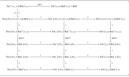
3. A CaseStudy
queue on channelinand dequeuing values by outputting on channelout.
Buff def= in?y.allocz. Frnkb!zkc1!(y,z)
k c1?(y,z).out!y. Bckkd!z
Frn def= recw.b?x.in?y.allocz. wkb!zkx!(y,z)
Bck def= recw.d?x. x?(y,z).out!y. wkd!z
In order to decouple input requests from output requests while still preserving the order of inputted values, the process handling inputs in Buff,in?y.allocz. Frnkb!zkc1!(y,z)
, stores inputted val-ues v1, . . . ,vnas a queue of interconnected outputs
c1!(v1,c2) k . . . k cn!(vn,cn+1) (3.1)
on the internal6channels c1, . . . ,cn+1. The process handling the outputs, c1?(y,z).out!y. Bckkd!z,
then reads from the head of this queue,i.e., the output on channel c1, so as to obtain the first value
inputted, v1, and the next head of the queue, c2. The input and output processes are defined in terms
of the recursive processes, Frn and Bck resp., which are parameterised by the channel to output
(resp. input) on next through the channels b and d.7
Since the buffer is unbounded, the number of internal channels used for the queue of intercon-nected outputs, (3.1), is not fixed and these channels cannot therefore be created up front. Instead, they are created on demand by the input process for every value inputted, using the Rπconstruct allocz.P. The newly allocated channel z is then passed on the next iteration of Frn through channel b, b!z, and communicated as the next head of the queue when adding the subsequent queue item; this is received by the output process when it inputs the value at the head of the chain and passed on the next iteration of Bck through channel d, d!z.
3.1. Typeability and behaviour of the Buffer. Our unbounded buffer implementation, Buff, can be typedwrt. the type environment
Γint def= in: [T]ω
,out: [T]ω
,b : [Trec] ω
, d : [Trec] ω
, c1: [T,Trec]• (3.2)
where T is the type of the values stored in the buffer and Trecis a recursive type defined as
Trec def
= µX.[T,X](•,1).
This recursive type is used to type the internal channels c1, . . . ,cn+1 — recall that in (3.1) these
channels carry channels of the same kind in order to link to one another as a chain of outputs. In particular, using the typing rules of Section 2 we can prove the following typing judgements:
in: [T]ω
, b : [Trec] ω
,c1: [T,Trec]1 ⊢in?y.allocz. Frnkb!zkc1!(y,z) (3.3)
out: [T]ω
,d : [Trec] ω
,c1: [T,Trec](•,1) ⊢c1?(y,z).out!y. Bckkd!z (3.4)
From the perspective of a user of the unbounded buffer, Buffimplements the interface defined by the environment
Γext def= in: [T]ω
,out: [T]ω
abstracting away from the implementation channels b,d and c1.
6Subsequent allocated channels are referred to as c 2,c3,etc..
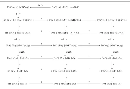
3.2. A resource-conscious Implementation of the Buffer. When the buffer implementation of Buffretrieves values from the head of the internal queue,e.g., (3.1), the channel holding the initial value,i.e., c1 in (3.1), is never reused again even though it is left allocated in memory. This fact
will repeat itself for every value that is stored and retrieved from the buffer and amounts to the equivalent of a “memory leak”. A more resource-conscious implementation of the unbounded buffer is eBuff, defined in terms of the previous input process used for Buff, and a modified output process, c1?(y,z).freec1.out!y.eBkkd!z, which uses the tweaked recursive process, eBk.
eBuffdef= in?y.allocz.Frnkb!zkc1!(y,z)
kc1?(y,z).freec1.out!y.eBkkd!z
eBkdef= recw.d?x.x?(y,z).freex.out!y. wkd!z
The main difference between Buffand eBuffis that the latter deallocates the channel at the head of the internal chain once it is consumed. We can typecheck eBuffas safe since no other process uses the internal channels making up the chain after deallocation. More specifically, the typeability of eBuffwrt.Γintof (3.2) follows from (3.3) and the type judgement below:
out: [T]ω
, d : [Trec] ω
, c1: [T,Trec](•,1) ⊢ c1?(y,z).freec1.out!y. Bckkd!z
Note that by the typing ruletIn of Figure 4, we need to typecheck the continuation of the input process,freec1.out!y. Bckkd!z
wrt. the type environment
out: [T]ω
, d : [Trec] ω
, c1: [T,Trec]•,y : T,z : Trec
where, in particular, c1is now assigned a unique channel type. According to the typing ruletFree, this suffices to safely type the respective deallocation of c1.
4. A Cost-BasedPreorder
We define our cost-based preorder as a bisimulation relation that relates two systems M ⊲P and
N⊲Q whenever they have equivalent behaviour and when, in addition, M⊲P is more efficient than N⊲Q. We are interested in reasoning about safe computations, aided by the type system described in Section 2. For this reason, we limit our analysis to instances of M⊲P and N⊲Q that are well-typed, i.e., that there exist (consistent) environments∆,∆′such that∆⊢M⊲P and∆′⊢N⊲Q. In order to preserve safety, we also need to reason under the assumption of safe contexts. Again, we employ the type system described in Section 2 and characterise the (safe) context through a type environment that typechecks it,Γobs. Thus our bisimulation relations take the form of a typed relation, indexed by type environments [21]:
Γobs(M⊲P)R(N⊲Q) (4.1)
Behavioural reasoning for safe systems is achieved by ensuring that the overall type environment (Γsys,Γobs), consisting of the environment typing M⊲P and N⊲Q, sayΓsys, and the observer environ-mentΓobs, is consistent according to Definition 2.2. This means that there exists a global environ-ment,Γglobal, which can be decomposed intoΓobsandΓsys; it also means that the observer process, which is universally quantified by our semantic interpretation (4.1), typechecks when composed in parallel with P,resp. Q (seetParof Figure 4).
typing environments. For instance, consider the two clients C0and C1we would like to relate from
the introduction:
C0,recw.allocx1.allocx2.srv1!x1.x1?y.srv2!x2.x2?z.c!(y,z).w
C1,recw.allocx.srv1!x.x?y.srv2!x.x?z.c!(y,z).w
(4.2)
Even though, initially, they may be typed by the same type environment, after a few steps, the derivatives of C0and C1must be typed under different typing environments, because C0 allocates
two channels, while C1only allocates a single channel. Our typed relations allows for this by
exis-tentially quantifying over the type environments typing the respective systems. All this is achieved indirectly through the use of configurations.
Definition 4.1 (Configuration). The tripleΓ⊳M⊲P is a configuration if and only ifdom(Γ) ⊆ M and there exist some∆such that (Γ,∆) is consistent and∆⊢M⊲P.
Note that, in a configurationΓ⊳M⊲P (whereΓtypes some implicit observer):
• c∈(dom(Γ)∪names(P)) implies c∈ Mi.e., M is a global resource environment accounting for both P andΓ.
• c∈ M and c<(dom(Γ)∪names(P)) denotes a resource leak for channel c.
• c<dom(Γ) implies that channel c is not known to the observer; in some sense, this mimics name scoping in more standardπ-calculus settings.
Definition 4.2 (Typed Relation). A type-indexed relationRrelates systems under a observer char-acterized by a contextΓ; we write
Γ M⊲PRN⊲Q
ifRrelatesΓ⊳M⊲P andΓ⊳N⊲Q, and bothΓ⊳M⊲P andΓ⊳N⊲Q are configurations.
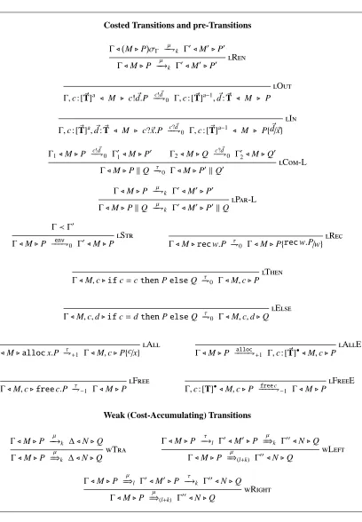
4.1. Labelled Transition System. In order to be able to reason coinductively over our typed rela-tions, we define a labelled transition system (LTS) over configurations. Apart from describing the behaviour of the system M⊲P in a configurationΓ⊳M⊲P, the LTS also models interactions between the system and an observer typed underΓ. Our LTS is also costed, assigning a cost to each form of transition.
The costed LTS, whose actions take the form −−→µ k, is defined in Figure 5, in terms of a top-level rule, lRen, and a pre-LTS, denoted as −−µ⇁k. The rule lRen allows us to rename channels for transitions derived in the pre-LTS, as long as this renaming is invisible to the observer, and is comparable to alpha-renaming of scoped bound names in the standard π-calculus. It relies on the renaming-modulo (observer) type environments given in Definition 4.3.
Definition 4.3 (Renaming ModuloΓ). LetσΓ : Name7→Namerange over bijective name substitu-tions satisfying the constraint that c∈dom(Γ) implies cσΓ=cσ−Γ1=c.
The renaming introduced bylRenallows us to relate the clients C0and C1of (4.2)wrt. an
ob-server environment such assrv1: [[T1]1]ω
,srv2 : [[T2]1]ω
of (1.6) and some appropriate common set of resources M even when, after the initial channel allocations, the two clients communicate potentially different (newly allocated) channels onsrv1. The rule is particularly useful when, later on, we need to also match the output of a new allocated channel onsrv2from C0with the output on
the previously allocated channel from C1 onsrv2. The renaming-modulo observer environments
function can be used for C1at that stage — even though the client reuses a channel previously
below for an explanation of how observers lose information. This mechanism differs from standard
scope-extrusion techniques for π-calculus which assume that, once a name has been extruded, it
remains forever known to the observer. As a result, there are more opportunities for renaming in our calculus than there are in the standardπ-calculus.
To ensure that only safe interactions are specified, the (pre-)LTS must be able to reason compo-sitionally about resource usage between the process, P, and the observer,Γ. We therefore imbue our type assumptions from Section 2 with a permission semantics, in the style of [42, 13]. Under this interpretation, type assumptions constitute permissions describing the respective usage of resources. Permissions are woven into the behaviour of configurations giving them an operational role: they may either restrict usage or privilege processes to use resources in special ways. In a configuration, the observer and the process each own a set of permissions and may transfer them to one another during communication. The consistency requirement of a configuration ensures that the guarantees given by permissions owned by the observer are not in conflict with those given by permissions owned by the configuration process, and viceversa.
To understand how the pre-LTS deals with permission transfer and compositional resource usage, consider the rule for output, (lOut). Since we employ the type system of Section 2 to ensure safety, this rule models the typing rule for output (tOut) on the part of the process, and the typing rule for input (tIn) on the part of the observer. Thus, apart from describing the communication of valuesd from the configuration process to the observer on channel c, it also captures permission~ transfer between the two parties, mirroring the type assumption usage in tOut and tIn. More specifically, rule (lOut) employs the operation c : [T]~ a−1 of Figure 4 so as to concisely describe the three variants of the output rule:
lOutU
Γ,c : [T]~ (•,i+1) ⊳ M ⊲ c!d~.P −−−c!⇁d~ 0 Γ,c : [~T](•,i), ~d :~T ⊳ M ⊲ P lOutA
Γ,c : [T]~ 1 ⊳ M ⊲ c!d~.P −−−c!⇁d~ 0 Γ, d :~ T~ ⊳ M ⊲ P lOutW
Γ,c : [T]~ ω
⊳ M ⊲ c!d~.P −−−c!⇁d~ 0 Γ,c : [T]~ ω
, ~d :T~ ⊳ M ⊲ P
(4.3)
The first output rule variant,lOutU, deals with the case where the observer owns a unique-after-(i+1) permission for channel c. Definition 4.1 implies that the process in the configuration is well-typed (wrt. some environment) and, since the process is in a position to output on channel c, ruletOut must have been used to type it. This typing rule, in turn, states that the type assumptions relating to the values communicated,d :~ T, must have been owned by the process and consumed by the output~
operation. Dually, since the observer is capable of inputting on c, ruletInmust have been used to type it,8which states that the continuation (after the input) assumes the use the assumptions d :~ ~T.
RulelOutU models these two usages operationally as the explicit transfer of the permissionsd :~ T~ from the process to the observer.
The rule also models the implicit transfer of permissions between the observer and the output process. More precisely, Definition 4.1 requires that the process is typedwrt. an environment that does not conflict with the observer environment, which implies that the process environment must have (necessarily) used an affine permission, c : [T]~ 1, for outputting on channel c.9In fact, any other
8More specifically,tInU of (2.9). 9This implies that
Costed Transitions and pre-Transitions
Γ⊳ M⊲Pσ
Γ
µ
−−⇁k Γ′⊳M′⊲P′
lRen Γ⊳M⊲P −−→µ k Γ′⊳M′⊲P′
lOut Γ,c : [~T]a ⊳ M ⊲ c!d~.P −−c!⇁0d~ Γ,c : [T]~ a−1, ~d :~T ⊳ M ⊲ P
lIn Γ,c : [T]~ a, ~d :T~ ⊳ M ⊲ c?~x.P −−c?⇁0d~ Γ,c : [~T]a−1 ⊳ M ⊲ P{d~/~x}
Γ1⊳M⊲P
c!d~
−−⇁0 Γ′1⊳M⊲P
′ Γ
2⊳M⊲Q
c?d~
−−⇁0 Γ′2⊳M⊲Q
′
lCom-L Γ⊳M⊲PkQ ⇁−τ0 Γ⊳M⊲P′kQ′
Γ⊳M⊲P −−⇁µ k Γ′⊳M′⊲P′
lPar-L Γ⊳M⊲PkQ −−⇁µ k Γ′⊳M′⊲P′kQ
Γ≺Γ′
lStr Γ⊳M⊲P −−−env⇁0 Γ′⊳M⊲P
lRec Γ⊳M⊲recw.P ⇁0−τ Γ⊳M⊲P{recw.P/w}
lThen Γ⊳M,c⊲ifc=cthenPelseQ ⇁0−τ Γ⊳M,c⊲P
lElse Γ⊳M,c,d⊲ifc=dthenPelseQ ⇁0−τ Γ⊳M,c,d⊲Q
lAll Γ⊳M⊲allocx.P ⇁−τ+1 Γ⊳M,c⊲P{c/x}
lAllE Γ⊳M⊲P −−−−alloc⇁+1 Γ,c : [~T]•⊳M,c⊲P
lFree Γ⊳M,c⊲freec.P ⇁−τ−1 Γ⊳M⊲P
lFreeE Γ,c : [T]•⊳M,c⊲P −−−−free⇁c−1 Γ⊳M⊲P
Weak (Cost-Accumulating) Transitions
Γ⊳M⊲P −−→µ k ∆⊳N⊲Q
wTra Γ⊳M⊲P =⇒µk ∆⊳N⊲Q
Γ⊳M⊲P −−→τ l Γ′⊳M′⊲P
µ
=⇒k Γ′′⊳N⊲Q
wLeft Γ⊳M⊲P =⇒µ(l+k) Γ′′⊳N⊲Q
Γ⊳M⊲P =⇒µ l Γ′⊳M′⊲P
τ
−−→k Γ′′⊳N⊲Q
[image:17.612.106.514.100.688.2]wRight Γ⊳M⊲P =⇒µ(l+k) Γ′′⊳N⊲Q
type of permission would conflict with the unique-after-(i+1) permission for channel c owned by the observer. Moreover, through the guarantee given by the permission used, c : [T]~ (•,i+1), the observer knows that, after the communication, it is one step closer towards gaining exclusive permission for channel c. RulelOutU models all this as the (implicit) transfer of the affine permission c : [~T]1 from the process to the observer, updating the observer’s permission for c to [T]~ (•,i)— note that two permissions c : [T]~ (•,i+1),c : [~T]1can be consolidated as c : [T]~ (•,i)using the structural rulestJoinand pUnqof Figure 4.
The second output rule variant of (4.3),lOutA, is similar to the first when modelling the explicit transfer of permissions d :~ ~T from the process to the observer. However, it describes a different implicit transfer of permissions, since the observer uses an affine permission to input from the configuration process on channel c. The rule caters for two possible subcases. In the first case, the process could have used a unique-after-(i+1) permission when typed usingtOut: this constitutes a dual case to that of rulelOutU, and the rule models the implicit transfer of the affine permission c : [~T]1in the opposite direction,i.e., from the observer to the process. In the second case, the process could have used an affine or an unrestricted permission instead, which does not result in any implicit permission transfer, but merely the consumption of affine permissions. Since the environment on the process side is existentially quantified in a configuration, this difference is abstracted away and the two subcases are handled by the same rule variant. Note that, in the extreme case where the observer affine permission is the only one relating to channel c, the observer loses all knowledge of channel c.
The explicit permission transfer forlOutW of (4.3), is identical to the other two rule variants. The use of an unrestricted permission for c from the part of the observer, c : [T]~ ω
, implies that the output process could have either used an affine or an unrestricted permission—see (2.5). In either case, there is no implicit permission transfer involved. Moreover, the observer permission is not consumed since it is unrestricted.
The pre-LTS rulelIncan also be expanded into three rule variants, and models analogous per-mission transfer between the observer and the input process. Importantly, however, the explicit permission transfer described is in the opposite direction to that oflOut, namely from the observer to the input process. As in the case oflOutA of (4.3), the permission transfer from the observer to the input process may result in the observer losing all knowledge relating to the channels communi-cated,d.~
In order to allow an internal communication step through either lCom-L, or its duallCom-R (elided), the left process should be considered to be part of the “observer” of the right process, and vice versa. However, it is not necessary to be quite so precise; we can follow [19] and consider an arbitrary observer instead. More explicitly, the rule states that if we can find observer environments (Γ1 and Γ2) to induce the respective input and output actions from separate constituent processes making up the system, we can then express these separate interactions as a single synchronous interaction; since this interaction is internal, it is independent of the environment representing the observer in the conclusion,Γ. See [19] for more justification.
a cost are those describing allocation and deallocation, where the respective costs associated are inherited directly from the reduction semantics of Section 2.
In Figure 5 we also specify weak costed transitions for configurations, based on the transitions of our LTS (rulewTra). As is standard, the relation denotes actions padded byτ-transitions to the left and right. However, it also accumulates the costs of the respective transitions into one aggregate cost for the entire weak action (ruleswLeftandwRight).
Technically, the pre-LTS is defined over triplesΓ,M,P rather than configurationsΓ⊳M⊲P, but we can prove that the pre-LTS rules preserve the requirements for such triples to be configurations; see Lemma 4.5.
Lemma 4.4 (Transition and Structure). Γ⊳M⊲P−−−µ⇁kΓ′⊳M′⊲P′and for∆consistent ∆⊢M⊲P implies the cases:
Ifµ=c!d: M~ = M′, k=0, P≡c!d~.P1 kP2, P′≡P1kP2 and Γ =(Γ′′,c : [T]~ a),
Γ′=(Γ′′,c : [~T]a−1, ~d : T) and ∆≺(∆′,c : [~T]b, ~d : T), (∆′,c : [T]~ b−1)⊢P′ for some P1,P2,Γ′′,b, ~T and∆′.
Ifµ=c?d: M~ = M′, k=0, P≡c?~x.P1kP2, P′≡P1{d~/~x} k P2 and
Γ =(Γ′′,c : [~T]a, ~d : T),Γ′ =(Γ′′,c : [~T]a−1) and ∆≺(∆′,c : [~T]b),
(∆′,c : [~T]b−1, ~d : T)⊢P′ for some P1,P2,Γ′′,b, ~T and∆′. Ifµ=τ: Either of three cases hold :
• M= M′, k=0 and Γ = Γ′ and ∆⊢P′or;
• M = (M′,c), k = −1 and P ≡ freec.P1 k P2, P′ ≡ P1 k P2,Γ = Γ′ and ∆≺∆′,c : [~T]• where∆′⊢P′(for some P1,P2, ~T and∆′) or;
• M′ =(M,c), k= +1 and P≡ allocx.P1k P2, P′ ≡ P1{c/x} kP2 andΓ = Γ′and∆≺ ∆′ and∆′,c : [T]~ • ⊢P′(for some P1,P2, ~T and∆′)
Ifµ=freec: M=(M′,c), k=−1 andΓ = Γ′,c : [~T]• and P=P′for someT.~
Ifµ=alloc: M′ =(M,c), k= +1 and Γ,c : [T]~ •= Γ′ and P=Q for some~T.
Ifµ=env: Γ≺Γ′, M= M′, k=0 and P= P′
Proof. By rule induction onΓ⊳M⊲P−−⇁µ kΓ′⊳M′⊲P′
Lemma 4.5 (Subject reduction). IfΓ⊳M⊲P is a configuration andΓ⊳M⊲P −−µ⇁k ∆⊳N⊲Q then ∆⊳N⊲Q is also a configuration.
Proof. We assume that dom(Γ) ⊆ M and that there exists ∆such that Γ,∆is consistent and that
∆ ⊢ M⊲P. The rest of the proof follows from Lemma 4.4 (Transition and Structure), by case analysis ofµ.
As a consistency check, we can also show that our LTS semantics is in accordance with the reduction semantics presented in 2. In particular, τ-transitions correspond to reductions modulo renaming and process structural equivalence.
Lemma 4.6 (Reduction and Silent Transitions).
(1) M⊲P−→k M′⊲P′impliesΓ⊳M⊲P
τ −
→kΓ⊳M′⊲P′′for arbitraryΓwhere P′′ ≡P′. (2) Γ⊳M⊲P→−τk ∆⊳M′⊲P′implies (M⊲P)σΓ−→k M′⊲P′for someσΓ.
Proof. By rule induction on M⊲P−→k M′⊲P′andΓ⊳M⊲P
τ
Example 4.7. Recall the buffer implementation Buff from Section 3 and the respective external environment Γext defined in Section 3.1. The transition rules of Figure 5 allow us to derive the
following behaviour for the configurationΓext⊳M,c1⊲Buff(wherein,out,b,d∈M):
Γext⊳M,c1⊲Buff
in?v1
−−−−→0 Γext⊳M,c1⊲
allocz. Frnkb!zkc1
![Figure 4. In fact, using the operation c : [T] (see Figure 4), ruleO collapses three differentpossibilities for typing output processes, which could alternatively have been expressed as the threeseparate typing rules in (2.8).](https://thumb-us.123doks.com/thumbv2/123dok_us/966743.609849/11.612.138.512.355.433/figure-operation-collapses-dierentpossibilities-processes-alternatively-expressed-threeseparate.webp)