Domain modelling for ubiquitous computing applications

Domain Modelling for Ubiquitous Computing Applications

Anthony Harrington and Vinny Cahill

Distributed Systems Group

School of Computer Science and Statistics

Trinity College Dublin

E-mail:

[email protected]

Abstract

Many Ubiquitous computing applications can be consid-ered as planning and acting problems in environments char-acterised by uncertainty and partial observability. Such systems rely on sensor data for information about their en-vironment and use stochastic or probabilistic reasoning al-gorithms to infer system state from sensor data.

We propose a domain modelling technique that charac-terises the sensor and actuator infrastructure and the set of system states in Ubicomp application domains. We capture the location and geometry of all domain model elements and use these spatial properties to tailor system state determi-nation to reflect the quality and spread of the sensor and actuator platform.

The domain model is used to support the development of Ubicomp applications and allows us calculate the degree of observability that exists over the state space in the envi-ronment. The degree of observability over the state space can act as an input into determining the state inference and action selection algorithms used in Ubicomp systems.

In this paper we present the design of our Ubicomp do-main model. We show that the proposed model contains information necessary to support Ubicomp application de-velopment. The expressiveness of the proposed design has been tested by building a model of an Urban Traffic Control application for Dublin city.

1

Introduction

Many Ubiquitous computing (Ubicomp) applications can be considered as real world planning and acting prob-lems. Canonical examples of such applications are the control of transportation infrastructures, activities such as region-wide pollution monitoring and emergency service management.

Ubicomp applications can be modelled as a set of sys-tem goals, actions that the syssys-tem is capable of taking and the decisions that must be taken to achieve the desired out-come or state. The set of actions associated with Ubicomp applications is bounded by the functionality of the actuator infrastructure deployed in the environment or application domain. Ubicomp applications are also optimisation prob-lems in so far as they attempt to maximise or minimise some property of the environment.

Partial observability is a challenging characteristic that real world environments present as application domains and stems from the dependence on sensor data for state deter-mination with the attendant possibility of error or partial coverage in the sensor readings. The sensor platform sits between the application and the environment thereby pre-cluding full observability and global knowledge of system state. The uncertainty in state determination may require the use of stochastic or probabilistic reasoning algorithms that infer system state from sensor data [15].

Ubicomp applications acting in uncertain environments may be modelled using classical planning techniques that have been extended to explicitly model probabilistic state transitions and observations [4]. These applications use control or optimisation algorithms for choosing actions for changing the state of a system so that it moves towards its desired goal state.

An important result from optimisation theory are theNo Free Lunchtheorems [17] that state that there is no one sin-gle optimisation strategy or algorithm that is optimum over the set of all possible problems. These theorems imply that the choice of optimisation strategy in Ubicomp applications should reflect the nature of the environment and the problem structure.

de-vising a solution and should be exploited where available [4] [11].

This analysis of Ubicomp applications indicates that properties of the application domain are very relevant when building such systems. We have developed a domain mod-elling process to support the profiling of Ubicomp domains and that can be used to support Ubicomp application devel-opment.

The proposed domain model is independent of an indi-vidual Ubicomp application and supports the development of multiple applications in a common domain. The principal requirement of the Ubicomp domain model is that it should contain the information necessary to model a Ubicomp ap-plication under development. The multi-layered domain model characterises the sensor and actuator infrastructure in the domain and the set of system states over which the application is defined. In a partially observable environ-ment the ability to determine the system state or the impact or efficacy of actions is dependent on the quality and spread of sensor infrastructure. Therefore the domain model must also support the development of an observation model that allows us to reason about the state of the system in uncertain environments.

To meet these requirements our domain model uses Ge-ographic Information Systems (GIS) support to allow state determination to reflect sensor and actuator position and spread. The domain model provides a uniform and scalable method of generating observation models that measure the quality of the sensor infrastructure and allows us to deter-mine where noise tolerant planning and optimisation strate-gies are appropriate.

The Ubicomp domain model is used to construct an ap-plication specific planning model. Our planning model is an application specific set of information extracted from a domain model and is a direct input into the development process.

This paper is structured as follows. In section II we for-malise the notion of a planning model for Ubicomp sys-tems and present the architecture of our domain model. In Section III we present the design of our domain model. In Section IV we present a case study of applying the do-main model to the development of an Urban Traffic Control (UTC) system in Dublin city and show how to construct a planning model from our domain model.

2

Domain Modelling and Planning for

Ubi-comp

In this section we formalise the notion of a Ubicomp planning model that encodes our knowledge of an applica-tion. We also present the architecture of our multi-layered domain model that stores the information necessary to con-struct a Ubicomp planning model.

The planning model is suitable for use in uncertain environments and is based on the standard model of state-transition systems [4]. It is a five-tuple P = (S, A, E, γ, O)where:

• S={s1, s2, ..}is a finite set of states;

• A={a1, a2, ..}is a finite set of actions;

• E={e1, e2, ..}is a finite set of events;

• γ:S×A×E→2s

represents a state-transition func-tion that may be non-deterministic to reflect a stochas-tic environment. If γ is non-deterministic and P is a probability distribution that represents the transition probabilities for each action in each state thenPa(s

′

|s)

is the probability that if we execute an actionain state s, thenawill lead to states′

.

• O = {o₁, o₂, ..} is a finite set of observations with probabilitiesPa(s|o), for anya ∈ A, s ∈ S ando ∈

O. Pa(s|o)represents the probability of observings after executing action aand receiving observation o. Observations are produced by the sensor infrastructure and identify the set of possible states the system might be in at each time step.

Ubicomp applications may be implemented using vari-ous components of such a planning model. The choice of optimisation technique applied in an application may be de-pendant on the information available to the developer. Con-sider the problem of optimising traffic flow in a city-wide region. Such an application if constructed as a Partially Observable Markov Decision Process (POMDP) would rea-son over observed belief states rather than the actual sys-tem state space [2]. If the application was constructed using a Reinforcement Learning algorithm the application would begin with no state-transition system and would attempt to learnγusing exploratory actions [1] [3]. Finally, if such a system were engineered using a Genetic Algorithm it would use a simulation of the system coupled with randomly se-lected state-space combinations to search for an acceptable solution to the problem [8]. The information required when building an application varies according to the choice of op-timisation algorithm employed by the designer.

Our first step when designing Ubicomp systems is to build a domain model that characterises important proper-ties of the domain. This domain model is used to construct a planning model specific to the application under devel-opment. The planning model is independent of the choice of optimisation algorithm that will be used. The goal is to use the information contained in the planning model as an input when selecting an appropriate optimisation algorithm during application development.

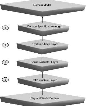
Figure 1. Layered Domain Model

service vehicle priority at traffic junctions. A domain model developed for the UTC domain will be useful for both ve-hicle priority and flow optimisation applications. With this consideration in mind, the domain model has been designed to be extensible and support many data formats. It is in-tended to provide a reusable basis for developing multiple applications in a domain.

2.1

Domain Model Architecture

The domain model is shown in Figure 1. There are four stages in the domain modelling process. The output of each stage is reflected in a layer of the domain model.

Layer 1 specifies the physical artifacts that exist in the application domain. The choice of relevant infrastructural elements is domain and application dependent. Physical artifacts relevant to the transportation domain include the location and geometry of transport network junctions and links, whereas office equipment and layout would be rele-vant artifacts in a smart office application.

Layer 2 specifies the functionality and spread of the sen-sor and actuator deployment in the application domain. This information contains the set of sensor states and actuator actions. The quality and spread of the sensor data will be used to determine the degree of observability over the sys-tem state space.

Layer 3 provides a higher-level partitioning of the do-main into system states that is more reflective of the applica-tion goals. Such states are typically composites of multiple sensor states.

Layer 4 of the domain model represents domain specific knowledge. Domain specific knowledge can act as a heuris-tic guide to a planning model for bounding the state-space

search in uncertain domains [4]. Domain knowledge may also be encoded in expert or rule based systems.

If no domain specific knowledge is available for an ap-plication then this layer of the model will be empty. In this scenario, a learning or stochastic search algorithm could be applied to optimise the system. Our approach is guided by the belief that if domain knowledge is present then we should utilise it. The use of elements in layers 1 to 3 is in-dependent of the presence or absence of domain knowledge in layer 4.

3

Domain Model Design

The principal requirements for the domain model design are that the model should contain the information necessary for constructing a Ubicomp planning model as described in Section II. It should also support the generation of obser-vation models that allow us to reason about the state of the system in uncertain environments.

The domain model classes are designed to map directly into the components of the planning model presented in Section II. Model elements are tagged with spatial attributes representing their location and geometry. Spatial attributes are used to match sensor and actuator positions to system states across regions of the domain and thereby determine the degree of observability over the set of system states.

3.1

Domain Model Abstractions

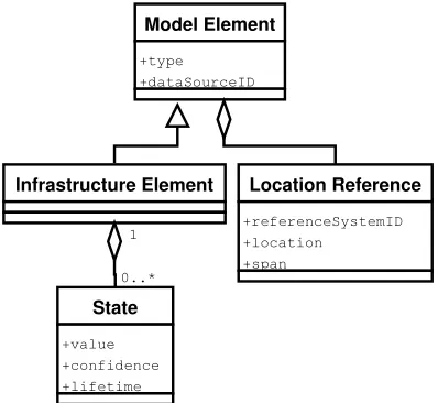
The domain model been designed using an object-oriented methodology. The Model Element is the base class from which all layer elements are derived. It contains two attributes: thetypeanddataSourceIdthat identify respec-tively the domain model layer to which the element belongs and the data format used to model the element. Layers 1 and 2 support a number of standard GIS data formats. Lay-ers 3 and 4 use XML schema to represent system states and domain specific knowledge.

The Location Reference class contains a referenceSys-temIdattribute that identifies the coordinate reference sys-tem used. Explicitly specifying the location referencing system used for each element allows model elements from separate layers to be overlayed and matched against each other. It also contains alocationattribute that specifies the physical location and geometry of elements in the domain model.

3.2

Domain Model Layers

3.2.1 Infrastructure Element Layer

Model Element

+type

+dataSourceID

Location Reference

+referenceSystemID

+location

+span

Infrastructure Element

State

+value

+confidence

+lifetime 0..*

1

Figure 2. Infrastructure Layer

1_{, Simple Features Specification for SQL (SFS)}2 _{and ESRI}

Shapefiles3_{. The design of this layer is shown in Figure 2.} In an Urban Traffic Control (UTC) scenario, infrastructure elements include road junctions and links. The spatial at-tribute of a road link element may be specified as a polygon object using a standard coordinate reference system. Like-wise the spatial attributes of a traffic light object may be represented using a point object.

3.2.2 Sensor/Actuator Layer

Layer 2 models the set of sensor states and actuator actions. The spatial attribute of a sensor includes both its physical lo-cation and sensing range. The design of this layer is shown in Figure 3.

The Sensor and Actuator elements derive from the Model Element. Both classes contain amobilityPattern at-tribute. Sensors and actuators may be stationary or mobile and the mobility pattern may impinge on system observabil-ity and optimisation algorithm selection. The Sensor class contains one or more State classes and the Actuator class contains zero or more State and one or more Action classes. In many applications the actions currently selected are also state information.

Elements of this layer contain aconfidenceattribute that indicates the degree of confidence associated with individ-ual sensor readings and is represented as a probability value between 0 and 1. This value represents a prior or uncon-ditional probability associated with the values produced by the sensor equipment.

1_{http://www.opengis.net/gml}

2_{http://www.opengeospatial.org/docs/99-049.pdf}

3_{http://www.esri.com/library/whitepapers/pdfs/shapefile.pdf}

Sensor

+mobilityPattern +return()

Model Element

+type +dataSourceID

Location Reference

+referenceSystemID +location

Actuator

+mobilityPattern +apply() +return()

State

+referenceArea +value +confidence +lifetime

Action

+referenceArea +value +confidence +lifetime 1

+* 1

*

0..1 *

Figure 3. Sensor Actuator Layer

A domain modeller could specify an inductive loop sen-sor [6] to have aconfidenceattribute of0.9whereas a virtual loop using video imagery may have a reducedconfidenceof

0.75. These values reflect the developers confidence in the sensor infrastructure in the domain.

3.2.3 System States Layer

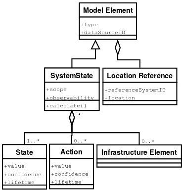
System States are composites of layer 1 and 2 elements. The set of system states are defined by the domain modeller and are usually derived from multisensor data.

The design of this layer is presented in Figure 4. Associ-ated with each system-state element arescopeand observ-ability attributes. Thescopeattribute defines the physical region over the domain model to which the system state re-lates and is expressed as a spatial value that can have one of three values:

• Infrastructure Element Scope. A system state can be defined at the level of an individual element at the infrastructure layer with a location reference attribute that matches the associated infrastructure element lo-cation reference.

• Multiple Element Scope. A system state can be de-fined at the level of multiple infrastructure elements. The location reference attribute of such a system state is the minimum-bounding-rectangle of the multiple el-ements.

Model Element

+type +dataSourceID

Location Reference

+referenceSystemID +location

SystemState

+scope +observability +calculate()

1..* 0..* *

0..* *

State

+value +confidence +lifetime

Action

+value +confidence +lifetime

Infrastructure Element

Figure 4. System States Layer

Theobservabilityof a system state is a measurement of the sensor spread and quality in the region of the domain model determined by the scope of the system state element. It is related to the confidence level associated with sensor readings relating to its constituent layer 2 elements.

The set of possible system states is constrained by the elements defined at layer 1 and 2 as it is only possible to de-fine a system state over the existing elements of the under-lying layers. By defining a system state, the modeller iden-tifies the type of infrastructure and sensor and actuator layer data that is relevant to determining the value of the system state. The mapping from element type to the deployed sen-sor and actuator platform in the application environment is performed using spatial operations over the geometries as-sociated with all layer elements.

This mapping or registration between sensor and actua-tor components and system states is used to support multi-sensor integration and fusion.

3.2.4 Domain-Specific Knowledge Layer

Layer 4 represents domain specific knowledge as pre-specified action selection strategies that map relationships between model components that have been identified by the developer. This knowledge is encoded in the state-transition system.

An example of domain specific knowledge in the UTC domain is the traffic theory governing the relationship be-tween optimum cycle time at a junction and flow rate at approaches to the junction [16].

In the absence of this domain knowledge or mapping we would have to use search and exploration techniques to learn this relationship. In a complex real world system the

state-space size might be large enough to render such a task prohibitive, as evidenced in [8].

3.3

Observation Model

The observation model characterises the efficacy of the sensor and actuator infrastructure when determining system state and can be used as an input into multisensor integra-tion and fusion techniques.

Multisensor integration and fusion involves high-level challenges such as the integration of multiple sensors at the system architecture and control level to more specific issues - possibly mathematical or statistical involved in the actual combination of multisensor information [10].

This challenge may be decomposed into three sub tasks: sensor selection, data fusion and estimation or inference about the system state. Layer 3 elements in the domain model contain a spatial mapping between a system state and its related set of sensor and actuator data. This mapping is used to support sensor selection. Theconfidenceattribute associated with sensor and actuator data can act as an input into sensor fusion and state inference techniques.

The choice of fusion and inference algorithms used in Ubicomp application development is independent of the proposed domain and planning model.

A Ubicomp application constructed as a POMDP will use an observation model to construct a belief state which is a probability distribution over all possible system states. This belief space is then used when determining action se-lection [12]. Another approach is to use Dynamic Bayesian Networks for sensor fusion and state inference. Sensor data may be represented as evidence or observation nodes in a Bayesian network and the sensorconfidence attribute can be used in determining a weighting for the associated ev-idence nodes [7]. In this scenario action selection is then based on an inferred system state rather than an observed belief state [13].

The use to which the information contained in the obser-vation model is put, is related to the choice of optimisation algorithm for the application.

4

Domain Model Implementation

We have applied our domain modelling process to the UTC application domain and have constructed a model of the SCATS UTC system [14] that is deployed in Dublin City Centre. We have used the uDig geospatial platform4_to de-velop a domain modelling tool. This tool provides the GIS support required to perform spatial operations that match sensor and actuator position and readings to system state scope. Layer 1 and 2 elements are encoded using the SFS

Figure 5. Excerpt from UTC Infrastructure Layer

<<Sensor>>

Inductive Loop

+sensorElement +GML

+locationReference +fixed

+id +name +return()

<<Sensor>>

GPS Receiver

+sensorElement +GML

+locationReference +fixed

+id +name +return()

<<State>>

FlowRate

+linkReferenceArea +flowRate +confidence +lifetime

<<State>>

NumVehInRange

+junctionReferenceArea +vehInRange

+confidence +lifetime

Figure 6. UTC Sensor Elements

data format and layer 3 and 4 elements are encoded using XML schema. All model elements are tagged with spatial attributes based on the Irish National Grid Coordinate ref-erence system.

The Infrastructure Layer of our domain model contains Traffic Junction and Road Link elements that represent the road network in Dublin. Fig 5 shows a screen shot of Infras-tructure Layer elements from a region of the road network adjacent to Trinity College in Dublin.

In addition to capturing the geometry and structure of the network, the Junction element specifies the set of traffic light phases or control sequences that can run at a junction and the Link element specifies the maximum rate at which vehicles can flow along the link. This value has been es-tablished from traffic theory to be 1800 vehicles per hour [16].

<<Actuator>> Traffic Controller

+actuatorElement +GML +locationReference +fixed +id +name +apply() +return()

<<State>> Phase

+junctionReferenceArea +phase

+phaseLength +confidence +lifetime

<<State>> CycleLength

+junctionReferenceArea +cycleLength +confidence +lifetime

<<Action>> SwitchPhase

+junctionReferenceArea +phaseId +confidence +lifetime

<<Action>> AlterCycleLength

+junctionReferenceArea +cycleLength +confidence +lifetime

Figure 7. UTC Actuator Elements

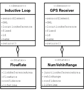
Fig 6 shows two Sensor elements from Layer 2 of the model. The Inductive Loop and GPS Receiver sensors pro-vide sensor data on the flow rate of a link and the number of vehicles in range of a junction respectively.

Fig 7 shows an Actuator element from Layer 2 of the model. The Traffic Controller actuator provides data on the current control phase and cycle-length at a traffic light junc-tion. This actuator can act to switch phases and to alter the junction cycle length.

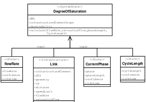
Fig 8 shows theDegreeOfSaturationsystem state from Layer 3 of the model. This system state is used by the op-timisation strategy employed by SCATS application to con-trol the traffic light settings in the UTC system [9]. It is a composite of Layer 1 and Layer 2 elements and is defined as:

x=q/Q

qis the actual flow rate in vehicles/hour;Qis the maximum achievable flow of an approach to a signal and is calculated fromQ= sg/C;sis the saturation flow or the maximum rate at which traffic can flow along the link;gis the green time allocated to a traffic light control phase and Cis the cycle time in operation at the traffic light junction.

This system state captures the ratio of effectively used green time to available green time at a junction. The SCATS policy is to keep this ratio at 0.9, i.e. traffic should flow through a junction for 90% of the portion of a green phase. TheDegreeOfSaturation (DOS)on a link may be calculated as :

f lowRate/saturationF low×phaseLength cycleLength

This components of this system-state are:

• flowRate- a layer2 element

• saturationFlow- a layer 1 infrastructure element

<<SystemState>> DegreeOfSaturation

+XML

+infrastructureElementScope +observability

+calculate(flowRate,saturationFlow,phaseLength, CycleLength)

<<State>>

flowRate

+flowRate +confidence +lifetime

<<State>> CurrentPhase

+phase +phaseLength +confidence +lifetime <<Infrastructure>>

Link

+infrastructureElement +SFS

+geometry +id +distance +speedLimit +flowRate +saturationFlow

input input

<<State>> CycleLength

+cycleLength +confidence +lifetime

Figure 8. Sample UTC System States Layer

• cycleLength- a layer 2 element

SCATS uses theDOSsystem state as a metric for cal-ibrating traffic light junction cycle times to maximise the throughput of traffic at a junction. A traffic junction has a number of approaches and SCATS calculates aDOSvalue for each approach to the junction.

In our domain model we assign eachDOSsystem state an infrastructure element scope that matches the geometry of the road link element specified in layer 1. The overlap-ping spatial attributes allow us to identify the actual set of sensors and actuators deployed in the environment that are associated with each separate instance of theDOSsystem state on each approach to all junctions in the system. Once the sensors and actuators have been identified, the possibly varying degree of observability over a set of common sys-tem states can be calculated and used in sensor fusion and state inference techniques.

From traffic theory [16] the relationship between the op-timum junction cycle timeCand traffic flowY is:

C= (1.5L+ 5)/(1−Y)

Y is the total flow ratio and is calculated asPywhere y is defined as the movement flow ratio y = q/swhere q is the demand or flow rate on an approach and sis the saturation flow or the maximum rate at which traffic can pass a point. Lis the lost time for a signal intersection due to safety delays between phase switching.

By exploiting this domain specific knowledge the system can apply a control strategy to optimise traffic flow by alter-ing junction cycle length times in response to variations in traffic flow.

4.1

Building a Planning Model

The domain model is parsed to extract the information required to construct a planning model. This process in-volves iterating over the set of system states to determine the infrastructure layer and sensor and actuator layer ele-ments that are relevant to the application.

Algorithm 1Parsing the Domain Model

Input: D{a Ubicomp domain model}

1: for allsystem statesdo

2: select layer1 and 2 elements within scope

3: calculate associatedconfidenceattributes

4: seed state inference algorithms withconfidence at-tributes

5: populate the setsSandAof states and actions

6: end for

Step 2 is implemented using the GIS platform. The regis-tration of sensors and their associated confidence attributes facilitates multisensor integration and fusion algorithms.

In the UTC domain model theflowRatesensor reading is associated with the(DOS)system state. This reading is ob-tained from inductive loop sensors located along each road Link element. In this application there is a one to one map-ping between the inductive loop sensor and theflowRatefor each traffic light phase at all Junction elements. In this case there is no requirement for multisensor integration or fu-sion.

5

Conclusions

The proposed domain modelling technique has been de-veloped to support Ubicomp development in environments characterised by partial observability. The domain model captures the information required to construct a planning model that acts as an input into the Ubicomp development process.

System states are defined as composites of the sensor, ac-tuator and infrastructure layer elements. An application is defined across a subset of system states. All model elements are tagged with spatial attributes to automate the registration or association of deployed sensors and actuators to system states. This information coupled with the prior probabilities associated with sensor readings can support multisensor in-tegration and fusion techniques that allow us to determine the degree of observability that exists over the set of system states.

sets that are required to represent the infrastructure and sen-sor and actuator elements in the city region. However a lot of this data is available is standard geographic data formats from the City Council authorities. The multi-layer mod-elling approach and spatial operations provide a uniform and scalable method of evaluating the sensor coverage in Ubicomp domains.

We now wish to build domain models for a range of Ubi-comp domains and explore how the planning model and observability metrics can be used as an aid in identifying appropriate optimisation algorithms for Ubicomp applica-tions.

References

[1] B. Abdulhai, R. Pringle, and K. G. Reinforcement Learning

for True Adaptive Traffic Signal Control. Transportation

Engineering., 129(3), May 2003.

[2] A. R. Cassandra, L. P. Kaelbling, and M. L. Littman. Act-ing optimally in partially observable stochastic domains. In

Proceedings of the Twelfth National Conference on Artificial Intelligence (AAAI-94), volume 2, pages 1023–1028, Seat-tle, Washington, USA, 1994. AAAI Press/MIT Press. [3] J. Dowling, R. Cunningham, A. Harrington, E. Curran, and

V. Cahill. Emergent consensus in decentralised systems us-ing collaborative reinforcement learnus-ing. In O. Babaoglu, M. Jelasity, A. Montresor, C. Fetzer, S. Leonardi, A. van

Moorsel, and M. van Steen, editors,Post-Proceedings of the

workshop SELF-STAR: Self-* Properties in Complex Infor-mation Systems, Hot Topics in Computer Science, volume

3460 ofLecture Notes in Computer Science, pages 63–80.

Springer-Verlag, May 2005.

[4] M. Ghallab, D. Nau, and P. Traverso. Automated Planning

Theory and Practice. Morgan Kaufmann, 2004.

[5] L. Klein. Sensor Technologies and Data Requirements for

ITS. Artech House, 2001.

[6] K. Korb and A. Nicholson. “Bayesian Artificial

Intelli-gence”. Chapman and Hall, 2004.

[7] H. Lo and A. Chow. Control Strategies for Over-Saturated

Traffic.Transportation Engineering., 130(4), 2004.

[8] P. Lowrie. “The Sydney Co-ordinated Adaptive Traffic

Sys-tem - principles, methodology, algorithms”. InProc. IEEE

International Conference on Road Traffic Signalling, pages 67–70, 1982.

[9] R. Luo and M. Kay. “Multisensor Integration and Fusion in

Intelligent Systems”. IEEE Transactions on Systems, Man,

and Cybernetics, 19(5), September/October 1989.

[10] M. Maurette. Mars rover autonomous navigation. Auton.

Robots, 14(2-3):199–208, 2003.

[11] S. Russell and P. Norvig. Artificial Intelligence - A Modern

Approach. Prentice Hall, 2 edition, 2003.

[12] A. Senart, M. Bouroche, G. Biegel, and V. Cahill. A

component-based middleware architecture for sentient

com-puting. InECOOP 2004 Workshop on Component-Oriented

Approaches to Context-Aware Systems, June 2004.

[13] A. Sims and K. Dobinson. “The Sydney Co-ordinated Adap-tive Traffic System (scat) System Philosophy and Benefits”. InProc. IEEE International Conference on Vehicular Tech-nology, volume VT-29, pages 130–137, 1980.

[14] J. Spall.Introduction to Stochastic Search and Optimization.

Wiley InterScience, 2003.

[15] F. Webster.Traffic Signal Settings - Technical Paper No 39.

Road Research Laboratory, London, UK, 1959.

[16] D. H. Wolpert and W. G. Macready. No free lunch

theo-rems for optimization. IEEE Transactions on Evolutionary