Abstract—In this paper, the traditional Π equivalent circuit
used to model the transformer is replaced by an ideal model in discrete optimal power flow (DOPF) formulation, which introduces a fictitious bus to express the power and voltage converting relations of the tap-changing transformer, so the admittance matrix is fixed during iterations to reduce computational efforts. Furthermore, this representation of transformer helps DOPF problem to be decoupled into two subproblems, which can improve computational efficiency greatly. Interior point method is used to solve continuous active power subproblem, and interior point cutting plane method (IPCPM) is adopted to solve discrete reactive power subproblem. Unfortunately, we find that the convex combination solution appears with great probability when solving DOPF problem, so in this paper IPCPM is improved to repair this shortcoming. Numerical simulations on IEEE14~300 test systems show that the improvement of IPCPM is efficient, and the proposed method is suitable for solving DOPF problems for large-scale systems.
Index Terms— Discrete Optimal Power Flow; Decoupled Optimal Power Flow; Interior Point Method; Interior Point Cutting Plane Method 1
I. INTRODUCTION
A key requirement of any modern society is the economic and secure operation of its electric power system. Such an important objective naturally demands the use of advanced large-scale system analysis, optimization, and control technologies. As a most attractive one of these technologies, optimal power flow (OPF) was proposed by Capentier in 1960s based on economic dispatch (ED) problem. Unlike ED that allocates load to the generating units only, the OPF integrates active and reactive power operation perfectly into one mathematical model via the AC load flow constraints around all buses, in which the economic and secure aspects of the concerned system are considered.
In recent decades, several classes of solution algorithms have been proposed to overcome OPF limitations in terms of flexibility, reliability and performance for real-world applications. However, these algorithms do not deal with the discrete step controls satisfactorily. On the other hand, such discrete controls are widely used by the power industry. For example, transformers are used for voltage control, shunt
1 Manuscript received Novenber 9, 2006. This work was supported by
special fund of the national priority basic research of China (2004CB217905)
.
Ding Xiaoying is with the Xi’an Jiaotong University, Xi’an, 710049, P.R.China (e-mail: [email protected])
Wang Xifan is with the Xi’an Jiaotong University, Xi’an, 710049, P.R.China.
Liu Lin is with the Xi’an Jiaotong University, Xi’an, 710049, P.R.China (e-mail: [email protected])
capacitors and reactors are switched on or off in order to correct the voltage profile and reduce transmission losses, and phase shifters are used to regulate the MW flow of transmission lines. So an efficient and effective OPF discretization procedure is needed to help the operators utilize these discrete controls in realistic and optimal manner. Exact modeling of discrete controls together with continuous control variables makes the OPF become a mixed integer nonlinear programming problem. The combinatorial-search approaches, branch-and-bound and cutting-plane method are usually used to solve this kind of mixed-integer programming model [1,2], but these methods are “nonpolynomial”, and all suffer from the so-called problem of “curse of dimensionality” for large-scale applications, making them unsuitable for larger-scale discrete OPF (DOPF) problems. Global optimization techniques, such as genetic algorithm (GA)[3,4], simulated annealing (SA)[5], tabu search (TS)[6], evolutionary programming and evolutionary strategy [7,8] have been applied to DOPF problem, which improve solutions but have relatively slow performance and unstable optima. Recently, due to the basic efficiency of interior point methods, which offer fast convergence and convenience in handling inequality constraints in comparison with other methods, interior point (IP) linear programming [9], quadratic programming [10], and nonlinear programming [11] methods have been widely used to solve OPF problem of large-scale power systems. However, up to now the interior point methods cannot directly solve the mixed-integer programming because gradient information is necessary. Liu et al. [12] extends the primal-dual IP algorithms to handle the discreteness of switchable shunt capacitors/reactors and tap-changing transformers in solving nonlinear reactive-power optimization by incorporating a positive-curvature quadratic penalty function in iterations. In 2004, interior point cutting plane method (IPCPM) was first applied to solve high-dimension nonlinear mixed-integer OPF problems [13]. All these improvements in IP algorithm encourage the successful implementation for rigorous solution of DOPF problem.
The traditional Π equivalent circuit used to model the transformer is replaced by an ideal model in this paper. The limitation of Π transformer model is that the change of tap setting requires repeated calculation of admittance matrix in iterations, which can greatly increase the computational efforts of algorithm. In the proposed formulation, the fictitious buses are added to express the power and voltage converting relations of the tap-changing transformer. So the admittance matrix is fixed in iterations to reduce computational efforts. Furthermore, the new representation of transformer helps DOPF problem to be decoupled into two subproblems
Interior Point Cutting Plane Method for
Discrete Decoupled Optimal Power Flow
completely. The advantages of the decoupled OPF formulation include: (1) decoupling greatly improves computational efficiency, especially for larger systems. It is because that each subproblem has approximately half the dimension of the original problem; (2) decoupling makes it possible to use different optimization techniques to solve the active power and reactive power OPF subproblems. In this paper, IP method is used to solve continuous active power subproblem (P-subproblem), and IPCPM is adopted to solve discrete reactive power subproblem (Q-Subprobelm). Numerical simulations on IEEE14~300 test systems show that the proposed method is efficient in solving OPF problems for large-scale power systems.
IPCPM is a hybrid of cutting plane method and IP method, which obtain good performance from these two methods. Although there are some papers on IPCPM application to several well known combinatorial optimization problems, such as linear ordering problem [14], flowshop scheduling problem [15] etc. IPCPM is first applied to solving high-dimension nonlinear mixed-integer OPF problems in 2004. Numerical simulations on IEEE 14~300 buses test systems show that the IPCPM is suitable for solving discrete optimization problems of large-scale systems. Currently, our observation is that IPCPM cannot obtain the correct information to identify optimal basis when the linear programming relaxation of original integer programming is a multiple-optima problem. Thus ambiguous information may increase the iteration numbers and computational time, even makes IPCPM completely fail. In this paper, IPCPM used in [13] is improved, the optimal solution shifting helps to ensure the generation of effective cutting plane constraints in the solution of the multiple-optima problems.
II. THE FORMULATION OF DOPF
A. The ideal model of Tap-changing Transformer
OPF problem is a difficult problem in mathematical programming area due to its large dimension, discrete and nonlinear characteristics when discrete controls are considered, such as tap-changing transformers, switchable shunt capacitors/ reactors, feasible AC transmission systems (FACTS) etc. In paper [13], an efficient integer programming approach, IPCPM is used to solve DOPF problems, and its calculation flow shows that the admittance matrix must be calculated with the improved tap setting in each iteration, which consists main computational burden of algorithm. This suggests that a good part of the computational work could be bypassed if the relationship between the transformer tap setting and the admittance matrix are eliminated. The best way we found to do so is to introduce a fictitious bus into the transformer model, which would be used to express the power and voltage converting relations of the tap-changing transformer.
As an example, tap-changing transformer branch is used to show a mathematical interpretation of the two different
model (see Fig.1). Where i and jare the head and end bus of
transformer branch separately, and non-standard voltage ratio side is jside. The traditional Π equivalent circuit model is
illustrated in Fig. 1 (a), and the model we used in this paper is shown in Fig.1 (b), where j,i′,iare high voltage bus, fictitious
bus and low voltage bus separately.
In Fig.1 (b), for fictitious bus i′, PTi′i can be described as flowing:
) sin cos
(
2
i i T i i T i i T i i i
T V g V V g b
P ′ = ′ − ′ θ′ + θ′ (1)
Due toPTi′i=PTji′, equation (1) can be rewritten as: ) sin cos
(
2
i i T i i T i i T i i
Tj V g VV g b
P ′= ′ − ′ θ′ + θ′ (2)
In addition, we obtain the following relations as the (1) analogue:
T i i i T i i T i i i
Tj V V b g V b
Q ′= ′ ( cosθ′ − sinθ′)− 2′ (3)
) sin cos
(
2
i i T i i T i i T i i
Ti V g VV g b
P ′= − ′ θ′ − θ′ (4)
T i i i T i i T i i i
Ti V V b g V b
Q ′= ′ ( cosθ′ + sinθ′)− 2 (5)
Furthermore, we know: i j=θ′
θ (6) i
j V
V
k= ′ (7)
From the expression collected in Table 1, one can see that the action of transformer tap is replaced by the voltage of fictitious bus when using the model in Fig1 (b). We can omit the computational burden for admittance matrix in iterations.
B. The Formulation of DOPF Problem
The DOPF problem can be decomposed into two subproblems, the continuous P-subproblem and discrete Q-subproblem with the transformer model in Fig2 (b). These two suproblems can be stated as follows.
i. P-subproblem
Objective function (operation cost minimization):
min ( 2 Gi2 1i G 0i)
SG i
iP a P a
a + +
∑
∈(8) Equality constrains:
∑
∑
∈ ∈
+ =
−
St ij
Tij Sl
ij Lij Di
Gi P P P
P
(9)
i j=θ′
θ
(10) Inequality constraints:
(a) Upper and lower bounds on the active power: max
min Gi Gi
Gi P P
P ≤ ≤ (i∈SG) (11)
(b) Upper and lower bounds on the flow of transmission line: max
min Lij Lij
Lij P P
P ≤ ≤ (i,j∈Sl) (12) ii. Q-subproblem
Objective function (transmission losses minimization):
∑
∑
∈ ∈+ =
Δ
St sj
Tsj Sl
sj Lsj
S P P
P
Equality constrains:
∑
∑
∈ ∈
+ =
−
St ij
Tij Sl
ij Lij Di
Gi Q Q Q
Q (14)
i j k V V
t = ′
+γ
1 (k∈ST) (15) Inequality constraints:
(a) Upper and lower bounds on the reactive power: max
min Gi Gi
Gi Q Q
Q ≤ ≤ (i∈SG) (16)
(b) Upper and lower bounds on the magnitude of voltage in bus i:
max min i i
i V V
V ≤ ≤ (i∈SB) (17)
(c) Upper and lower bounds on the tap position i:
max min i i
i t t
t ≤ ≤ (i∈ST) (18)
Where: SB: the set of all buses, Sl: the set of all branches, St: the set of all transformer branches, SG: the set of all active sources, ST : the set of all tap-changing transformers,
i
a0 ,a1i,a2i: the fuel cost coefficients of unit i, PGi,QGi: active and reactive power generation at bus i, PDi,QDi: active and reactive demand at bus i, PLij,QLij: active and reactive flow in general branch
ij
, PTij ,QTij: active and reactive flow in transformer branch ij, ti: tap setting of tap-changing transformeri
, Vi,θi: the magnitude and angle of voltage in busi
, θij=θi−θj. •max,•min: the upper and the lower bounds on variables. γ : the adjust step of the kthtap-changing transformer. The other variables are described in sector 2.1.
III. THE CALCULATION FLOW OF ALGORITHM
The active power subproblem is described as (8)~(12),
which is a typical nonlinear programming problem. In this paper, it is solved by IP method (see [16], for the algorithm flow and formulations). IPCPM (see [13], for the principle and formulations of algorithm) is applied to solve the reactive power subproblem, which is a mixed integer nonlinear programming problem.
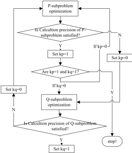
The proposed approach for DOPF problem is described in Fig 2 within the context of two optimization modules: the P-subproblem optimization and Q-subproblem optimization.
IV. THE IMPROVEMENT OF IPCPM
In cutting plane method, cutting plane constrains are available by the information of basis variables. An advantage of the conventional simple cutting plane method (SCPM) in getting a cut is that its optima of linear programming relaxation implicitly converges to the vertex of feasible region of problem in any cases. However, if the linear programming relaxation is multiple-optima problem, it is easy to prove that IPCPM cannot collect the correct information of optimal basis because its PTij+jQTij
PTi'j+jQTi'j
i j
i′
PTii'+jQTii'
1:k
gT+jbT
k YT
PTij+jQTij PTji+jQTji
i j
T
Y k k 1) ( −
T
Y k k
[image:3.595.102.501.97.193.2]2 ) 1 ( −
Fig.1 The equivalent circuit of transformer
(a) The traditional Π equivalent circuit model (b)The model used in this paper
Power
flow Π equivalent circuit model The ideal model
) (Tii TijP
P ′ i2T 1ViVj(gTcosij bTsin ij) k
g
V − θ + θ 2 ( cos sin )
i i T i i T i i T
ig VV g b
V − ′ θ′+ θ′
) ( Tii TijQ
Q ′ VjVibT ij gT ij VibT k
2 ) sin cos (
1 − −
θ
θ Vi′Vi(bTcosθii′−gTsinθii′)−Vi2bT
) (Tji TjiP
P ′ 12 j2T 1VjVi(gTcosij bTsin ij) k
g V
k − θ − θ ( cos sin )
2
i i T i i T i i T
ig VV g b
V′ − ′ θ′− θ′
) ( Tji TjiQ
Q ′ ji T ij T ij VjbT
k g b V V k
2 2 1 ) sin cos (
1 + −
θ
θ Vi′Vi(bTcosθii′+gTsinθii′)−Vi′2bT
[image:3.595.307.536.345.610.2]TABLE 1 THE POWER FLOW OF TRANSFORMER BRANCH IN TWO DIFFERENT MODELS
Fig.2 The calculation flow of DOPF problem P-subproblem
optimization
Set kp=1
Are kp=1 and kq=1?
Q-subproblem optimization
Is Calcultion precision of Q-subproblem satisfied?
Set kq=1
Set kp=0
Set kq=0
stop! Y
If kq=0
Y N
If kp=0
Y N Is Calcultion precision of
[image:3.595.44.295.605.701.2]optima of linear programming relaxation converges to an edge of feasible region of problem with a great probability. As a result, ambiguous basis information may increase the iteration numbers and computational time of IPCPM, even makes IPCPM completely fail.
A. The theoretic analysis
For clarification we assume that the following linear programming is the relaxation problem of mixed integer programming.
max. 2x1+4x2 (19) .
.t
s x1+2x2+x3=8 (20)
x1+x4 =8 (21)
x2+x5=8 (22) 0
, , ,
, 2 3 4 5
1 x x x x ≥
x (23)
The above linear programming is a multiple-optima problem, which have three kinds of solutions:
i. Normal solution: x′*=(2,3,0,6,0), that is to say, the number
of non-zero elements is equal to 3. It equals to the number of equality constraints.
ii. Degenerate solution:x′′*=(8,0,0,0,3), and the number of
non-zero elements is less than 3.
iii. Convex combination solution: * * (1 ) *
x x
x′′′ =α ′ + −α ′′ ,
where α∈(0,1) . For example, when
12 7
=
α ,
) 25 . 1 , 5 . 3 , 0 , 75 . 1 , 5 . 4 ( *= ′′′
x , and the number of non-zero elements
is more than 3.
The example in Fig.3 provides a geometrical interpretation of the three different kinds of solution when IP method is applied to solving problem (19)~(23). In Fig.3, the convex polytope ABDO is the feasible region of problem (19)~(23). Clearly, the constraint edge BD should parallel to the objective function (19). As a result, the maximum of objective function can be found in any point of edge BD, which explains the reason for the appearance of *
x′′′ . From Fig.3 we
can see, x′*=(2,3,0,6,0) is obtained when the algorithm
convergences to point B, or x′′*=(8,0,0,0,3) is obtained when
the algorithm convergences to point D, or
) 25 . 1 , 5 . 3 , 0 , 75 . 1 , 5 . 4 ( *= ′′′
x is obtained when the algorithm
convergences to point P stands between the point B and the point D.
For SCPM algorithm, simplex method(SM) is a vertex-searching method. It start at the origin, then it moves along the intersection of the boundary hyper-planes of the constraints, hopping from one vertex to the neighboring vertex, until an optimal vertex is reached. As a result, only two kinds of solution can be found, normal solution *
x′ and degenerate
solution *
x′′ (see Fig.3). x′′* can be transformed into x′* by
selecting some zero variable columns to enter the basis in accordance with some column selection criteria. That is to say, there is not much trouble of cut generation in SCPM, even in the presence of *
x′′ . Unlike SCPM, the IP method used in
IPCPM crosses the interior of feasible region in search for optima of linear program. Clearly, the probability of optima standing in edge BD is always much more than the probability of optima standing in point B or point D (see Fig.3). In other words, IP method found convex combination solution *
x′′′ with
a great probability in this case. If *
x′′′ is obtained, then IPCPM
cannot collect the correct information of optimal basis. Therefore, ambiguous basis information may increase the iteration numbers and computational time of IPCPM, even makes IPCPM completely fail. Unfortunately, we observe that this phenomenon occures frequently when we attempted to solve DOPF problem with IPCPM. So addressing above issue is key to the successful implementation of IPCPM for solving DOPF problem.
B. The improvement of IPCPM
The success of cut generation is dependent on the ability of the method to locate the normal solution *
x′ correctly and
effectively. Thus, it is obviously that transform *
x′′′ into x′* is
one of the important factors to solve the problem presented previously. When the optimum converges to an edge of feasible region of problem, it can be moved to the neighboring vertex by pivoting [17]. That is to say, the *
x′′′ can be transformed into
*
x′ with the following scheme.
We assume that the linear program relaxation
{
mincTxAx=b,x≥0}
(where c∈Rn,x∈Rn,A∈Rm×n,m
R ∈
b ) is solved by IP method, and xprimal and y,s dual
optimal solutions are available. Let A=
[
A1,A2,A3]
,[
x1,x2,x3]
x= , s=
[
s1,s2,s3]
,c=[
c1,c2,c3]
, where index 1 refers to the coordinates wherex
is positive, index 2 refers to the coordinates where both of x and s are zero, and finally index 3 refers to the coordinates wheres
is positive. Then wehave:A1x1=b,A1Ty=c1,AT2y=c2 and A3Ty<c3. Step1:Determine the kind of solution: (a) If it is *
x′ , then components of x′* corresponding to
zero element are said to be basic variables. Stop calculation. (b) If it is *
x′′ , go to Step7.
(c) If it is *
x′′′ , go to Step2.
Fig.3 The search route of IPM and SM
A
B
C
D P
x 0
* x′
x′′ *
x′′′ in te rio r p o in t m e th o d
Step2:Are the columns of A1 linearly dependent, if the answer is not go to Step6.
Step3:Pivoting: setx1′=x1+tz.
To guarantee the optimization of
x
: There must exist one but not only one vector z satisfying A1z=0 because thecolumns of A1 are linearly dependent, so any z is the one we need. (We can prove: The new objective function is
= + +
′ 2 2 3 3
1
1x c x c x
cT T T (A1Ty)T(x1+tz)+cT2x2+c3Tx3=c1Tx1
x c x c x c x c z A y x c x
cT + T +t T = T + T + T = T
+ 2 2 3 3 1 1 1 2 2 3 3 , so the
optimization of original problem solution does not be affected whenx1is transformed intox1′.)
To guarantee the feasibility of x: Compute tmin≤t≤tmaxby solving x1′=x1+tz≥0.
Step4:Eliminate zero element (say
j
) fromx1′ using mint or tmax. Remove ajfrom A1 and add toA2, then go to Step2.
Step5: Setx=[x1′,x2,x3], and then go to Step1.
Step6: SetB=A1, if rank(B)>rank([A1A2]) go to Step8. Step7: A column ajof [A1A2]is independent fromB, add j
a to B.
Step8: Go to Step11 if rank(B)=m.
Step9: Pivoting: Set y′=y−vu.
To guarantee the optimization of
y
: There is more than one vector u satisfying BTu=0, and any u is the one we need.(We can prove: The new objective function is bTy′=bTy−vbTu=bTy−vxTATu . It is clearly that
= u A
xT T
[
]
[
]
u 0A B 00 x u A A A x x x
3 = ⎥ ⎦ ⎤ ⎢ ⎣ ⎡ ′ = ⎥ ⎥ ⎥
⎦ ⎤
⎢ ⎢ ⎢
⎣ ⎡
′ 1
3 2 1
3 2
1 , so the optimization
of dual problem solution does not be affected when
y
is transformed into y′.).To guarantee the feasibility of y: Compute vmin≤v≤vmax by solvingA3Ty′≤c3.
Step10: Substitute vmin or vmax to y′=y−vu , and j
T
j c
a3 y′= 3 must exist. (where a3jrepresents the jth column of matrix A3, c3jis the jth component of vector c3). Remove
j
a3 from A3 and add toA2andB, then go to Step8. Step11: Stop, matrix
B
is the basis matrix that we need.V.
NUMERICAL SIMULATE AND ANALYSIS The proposed algorithm was implemented using the Visual C++6.0 language and the software program was executed on an 800-MHz Pentium Pro computer. Numerical simulations on RTS-24 test systems have been done to test the performance of the presented algorithm.A. The performance of proposed algorithm
In the proposed formulation, the fictitious buses are added to express the power and voltage converting relations of the tap-changing transformer. So the admittance matrix is fixed during iterations to reduce computational efforts. Furthermore, the new representation of transformer helps DOPF problem to be decoupled into two subproblems. The advantages of the decoupled OPF formulation include: (1) decoupling greatly improves computational efficiency, especially for larger systems. This is because each subproblem has approximately half the dimension of the original problem; (2) decoupling makes it possible to use different optimization techniques to solve the active power and reactive power OPF subproblems. In this paper, IP method is used to solve continuous P-subproblem, and IPCPM is adopted to solve discrete Q-subproblem.
From Table2, comparing with the algorithm proposed in paper [13], we find that the presented algorithm has attractive performance because its calculation speed enhances obviously during the scale of system becoming larger and larger. Based above analysis, we can conclude that the proposed method is very promising for solving discrete OPF problem, especially for large-scale power systems.
B. The improvement of IPCPM
Many numerical experiments have indicated that objective function of OPF has a very plain shape for the transformer tap control. Therefore, very similar cost values can be obtained with different settings of the transformer tap. So OPF becomes a multiple-optima problem. The same conclusion can be obtained form the numerical results illustrated in Table3, which shows that the convex combination solution appears with great probability when solving OPF problem (8)~(18) for IEEE14~300 test systems. Furthermore, It is seen in sector 3.1 that IPCPM has bad computational performance for multiple- optima problem. There is a need to extend IPCPM to repair this shortcoming. Table4 compares the performance of the two IPCPM for solving OPF problem, which shows that the proposed method is more efficient than its old version proposed in paper [13]. In summary, the improvements of IPCPM meet the needs of practical application, and it offers a new way to solve complicated discrete optimization problem for large-scale power system, which result in dramatic property and human save.
Model
Test system II model Ideal model
IEEE14 1359 359
RTS-24 2703 1062
IEEE30 5797 2578
IEEE57 10734 2625
IEEE118 26641 7359
IEEE300 77609 57125
VI. CONCLUSION
The OPF problem becomes a nonlinear mixed integer programming problem when the discrete controllers are considered, such as tap-changers in transformers or switching of capacitor/reactor banks and so on. It is proposed in this paper, that the traditional Π equivalent circuit used to model the transformer be replaced by an ideal model, which provides the following advantages:
(1) The admittance matrix is fixed in iterations to reduce computational efforts.
(2) The new representation of transformer helps DOPF problem to be decoupled into two subproblems, which improves computational efficiency.
On the other hand, in this paper, IPCPM is improved to meet the needs of practical application. Numerical simulations on IEEE14~300 test systems show that the proposed method is efficient in solving OPF problems of large-scale power systems.
REFERENCES
[1] E. C. Finardi, E. L. da Silva. Unit commitment of single hydroelectric plant. Electric Power Systems Research, 2005, vol. 75, pp: 116~123 [2] R.A. Jabr. Homogeneous cutting-plane method to solve the
security-constrained economic dispatching problem. IEE Proc.-Gener. Transm. Distrib. 2002, vol. 149, NO. 2, pp: 139~144
[3] Z. H. Wang, X. G. Yin, Z. Zhang, J. C.Yang. Pseudo-parallel genetic algorithm for reactive power optimization, IEEE Power Engineering Society General Meeting, 2003, vol. 2, pp:13~17
[4] S. Durairaj, Devaraj, P. S. Kannan. Improved Genetic Algorithm Approach for Multi-Objective contingency constrained Reactive Power Planning, INDICON, 2005 Annual IEEE, 2005, pp: 510~515
[5] Chen Haoyong, Wang Xifan. A Genetic Algorithm with Annealing Selection for Reactive Power Optimization. ZhongGuo Dianli/Electric Power, 1998, vol. 31, NO. 2, pp: 3~6
[6] Yutian Liu, Li Ma, Jianjun Zhang. GA/SA/TS Hybrid algorithm for reactive power optimization. IEEE Power Engineering Society Summer Meeting, 2000, vol. 1, pp: 245~249
[7] C. Jiang, C. Wang. Improved evolutionary programming with dynamic mutation and metropolis criteria for multi-objective reactive power optimization. IEE Proceedings on Generation, Transmission and Distribution, 2005, vol. 152, NO. 2, pp: 291~294
[8] C. C. A.Rajan, M. R. Mohan. An evolutionary programming-based tabu search method for solving the unit commitment problem, IEEE Trans. on Power Systems, vol. 2004, 19, NO. 1, pp: 577~585
[9] Chen Ji, Wei Hua. Application of an Improved Trust Region Interior Point Algorithm in OPF. Modern Electric Power. 2005, vol. 22, NO. 6, pp: 13~17
[10] Hua Wei, H. Sasaki, R. Yokoyama. An application of interior point quadratic programming algorithm to power system optimization problems. IEEE Transactions on Power Systems. 1996, vol. 11, NO. 1, pp: 260~266
[11] WEI Hua, LI Bin, HANG Nai-shan, et al. An implementation of interior point algorithm for large-scale hydro-thermal optimal power flow problem. Proceedings of the Csee. 2003, vol. 23, NO. 6, pp: 13~18 [12] Mingbo Liu, S. K. Yso, Ying Cheng. An extended nonlinear primal-dual
intwerior point algorithm for reactive-power optimization of large-scale power systems with discrete control variables. IEEE Trans. on Power Syetems, 2002, vol. 17, NO. 4, pp: 982~991
[13] X. Y. Ding, X. F. Wang, Y. H. Song. An interior Point Cutting Plane Method for Optimal Power Flow. International Journal of Management Mathematics, 2004, vol. 15, NO. 4, pp: 355~368
[14] J. E. Mitchell, B. Borchers. Solving Real-world Linear Ordering Problems Using a Primal-dual Interior Point Cutting Plane Method. Annals of Operations Research, 1996, vol. 62,pp.: 253~276
[15] Ding Xiao-ying, WANG Xi-fan, CHEN Hao-yong. A combined algorithm for optimal power flow. Proceedings of the CSEE, 2002, vol. 22, NO. 12, pp: 11-15
[16] Nimrod Megiddo, On Finding Primal and Dual Optimal Bases. Theory.Stanford. edu/~megiddo/pdf/primdual.pdf
system The dimension of matrix A
The number of non-zero elements
The number of zero elements
The type of optimum
5 24×28 25 3 *
x′′′
14 65×74 65 9 *
x′
24 114×132 118 14 *
x′′′
30 132×144 133 11 *
x′′′
57 243×258 245 13 *
x′′′
118 546×620 550 70 *
x′′′
300 1300×1400 1314 86 *
x′′′ TABLE.3 THE TYPE OF OPTIMUM OF DOPF PROBLEM
system The number of cuts The value of tap
Before improvement fail fail
5
After improvement 1 5
Before improvement 1 -4,-10
14
After improvement 1 -4,-10
Before improvement fail fail
24
After improvement 1 -2,-5,5
Before improvement 0 -10,-10,5,-5
30
After improvement 0 -10,-10,5,-5
Before improvement 0 -10,-5,-10,-5,10 57
After improvement 0 -10,-5,-10,-5,10
Before improvement fail fail
118
After improvement 1 -5,5,-5,0,-2,-5,5
Before improvement fail fail
300