Abstract— A posteriori optimization strategy for the local
adaptation of the regularization parameters for the nonlinear variational model in image motion is presented in this paper. The idea of such interesting method is based on the automatic step wise refinement of the solution with the special type of isotropic mesh refinement process which is controlled by a posteriori error estimate in a suitable norm which is a computable quantity and works as metric for the given domain refinement strategy and the determination of the optimized approximate solution in this paper. The main idea is to compute image motion with adaptive FEM (finite element method) based discretization of nonlinear variational problem then optimization with an interesting adaptive process which is a novel idea of optimization especially in the Imaging problems.
Index Terms— Finite Elements, Image Motion. Optimization, Isotropic mesh Adaption.
I. INTRODUCTION
The problems on the moving images are generally known as correspondence problems where one mainly is interested to compute the pixel shifts (disparities) during the moving image or camera shifts during the moving cameras. The main goal is therefore to compute the depth information of the scene. The determination of such disparities in formal terms is called optic flow problem. Main application of these problems is to distinguish the stationary from the moving objects; moreover the ideas of the image motion are very useful in the area of the robot navigation, medical imaging, video processing and also in the fluid mechanics etc. Generally these correspondence problems are inverse and ill-posed. The “inverse” and “ill-posed problems” have been surely gaining great popularity in mathematical sciences for last more than sixty years. The main interest in the study of such problems is their complexity and instable behavior. With the advent of the powerful computational technology, the inverse and ill-posed problems have attracted the mathematical community, especially the applications of such problems in imaging techniques have gained much attention [1]-[17].
The interesting and classical approaches for the solution of such problems is generally based on the idea of energy optimization and regularization, their history go back to the
Manuscript received 20th December 2018. This work was supported by Quqid-E-Awam University of Engineering, Science and Technology Nawabshah, Sindh-Pakista.
Khuda Bux Amur, Department of Mathematics and Statistics QUEST Nawabshah, Sindh-Pakistan (phone: +923468952131; e-mail: [email protected]).
Thikonov like regularization [5]. The problems in the computer vision and image processing research are usually ill-posed inverse problems. The regularization of the problems in PDE’s (Partial Differential Equations) based image processing is based on the idea of minimization of the energy functional [7]-[14]. These energy based regularization techniques in image processing generally depend on the optimal selection of the smoothing parameters. The usual choice of the regularization parameters in these techniques is a priori and uniform over the whole domain [11]-[14]. A new idea of non-uniform selection of scaling parameters was a priori and appeared as local iterative method for the denoising problem [6]. The novel method for the selection of regularization is based on the idea of a posteriori regularization was introduced for linear PDE’s based problems [3] and extended to the nonlinear problems by the author [7]. The further experiments were performed on a posteriori regularization as [8]-[10]. All the previous approaches [11]-[17] are based on the idea of optimization then discretization. This work is dedicated to the interesting idea of FEM based discretization then a posteriori optimization of the discrete solution which is of main interest in this work and a fresh contribution for the nonlinear variational problems. The special type of the mesh refinement yields the dramatic improvement in the solution of the coupled set of partial differential equations as a velocity image at each step of the computation.
II. OPTIMIZATION PROBLEM
The following nonlinear constraint optimization problem is proposed for the computation of two directional motions.
1 2 2
2
1 2 ( )
min(u)
(u)
1
2
t x x LT
subject to
f
f u
f u
(1)where
T
(u)
( )
x
2u d
2dx
representsthe convex regularization and the velocity vector
1 2
( ,
)
Tu
u u
describes the image motion in a video image sequence called optical flow. The
( )
x
0
continuous scaling function given on the domain
.
Herex
( ,
x x
2)
T andf
is image sequence designed as: ,
f where is two dimensional space domain. The terms
1
,
2x x t
f
f
and f
are denoted as the derivatives with respect tox
1,
x
2and t
. The optimization constraint given in problem (01) is directly obtained fromA Posteriori Optimization Process for the Local
Adaptive Smoothing in the Moving Images
the first order Taylors’s theorem on the following constancy assumption on the grey values of the of the moving image in the image sequence [12], [14]
f x x
( ,
1 2, )
t
f x
(
1
u x
1,
2
u
2,
t
1)
(2) The goal is to determine the two directional pixel velocities1 2
u(u u, )(ill-posed problem). The unconstraint settings for the above problems can be given by the following energy functional
2
1 2
2
1 2 ( )
u
1
min
(u)
2
t x x LT
f
f u
f u
(3)The first part of (03) T(u)called the smoothness term and the second term is called the data term. The solution of the given variational problem is given as
m
inf ( (u) : u
E
X )
(4) The problem (4) is solved as optimization problem in the space X of functions of the bounded variations in2. The existence of the minimizers of (03) follows from the direct methods of the calculus of variations. Since the smoothing term is convex and assuming that the dataf
is smooth enough. Applying the direct method of the calculus of variation, the minimization of the energy functional (03) yields the following Euler-Lagrange equations1 1 2 1
1 1 2 2
1 2 2 2 1 2 2 1 2 1 2 2 2 1 2 2 1 2 1 2 ( ( ) )
( ) 0
( ( ) )
( ) 0
0, on
x x x x t
x x x x t
u div x
u u
f u f f u f f u div x
u u
f u f f u f f
u u n n
(5) Set 1 2(
x t,
x t)
Tg
f
f
f
f
III. WEAK FORMULATION AND DISCRETIZATION
Weak formulation of (5) is give
1
2 2
2
1 2
1
( ) u : v
(
u v v v
Compute u H such that
x
dx
u u
J dx g dx H
(6)The problem is being discretized in the space
X
h
X
of1
P
finite elements, hereP K
1( )
denotes space of degree one polynomials in
2. The discrete domain is considered as triangular gridT
h with elements of maximum sizeh
0
.
0
1
: v ( ) , v ( )
h h h h K
X C KT P K
Discrete problem is given as
u
,
(u , v ; u ) (g, v )
v
hh h
h h h h
h h
h
Compute
X
b
X
here X
X
(7) 2 2 2 1 2( ) u : v
(u , v ; u )
(
u
v
(g, v )
v
h
h h
h h h
h h h h
x
b
dx
u
u
J
dx
g
dx
(8)The a posteriori optimization process for the initial optimized solution is based on the isotropic mesh adaptive procedure which is performed by a posteriori error estimates called residual error indicator [19] and the weight function
( ).
x
The residual error indicator for nonlinear variational model is defined in the spirit of [3, 7, 19].
2 2 2 2 1 2 2 , ( ) 1 1 2 2 ( )u
1
u
2
K K K h h h L K
e e e h e e L e e
h
g
J
h
n
(9)IV. COMPUTATIONAL STRATEGY AND NUMERICAL RESULT
The numerical experiments are performed using the FreeFem++ which is a programming language for the determination of FEM based solution of the PDE’s (Partial Differential Equations) [18]. We present the following a posteriori optimization adaptive process for the initial obtained solution (optic flow) in the spirit of [3, 7]
i. Compute minimizer of the problem (3)
u
0(initial optic flow) onT
0h with large
h.
ii. Perform adaptation and build new refined grid
T
h1using the metric as a posteriori estimate (9). iii.Set a local optimal choice for
h.
as new function1
h
and go to step ii to computeu
1 onT
h1. Such a choice of
hat each adaptive step is proposed as
1
max ( , ),
k
K K K Thr
(10) where max
(
,
)
1
(
0.1)
Where
Thr is a threshold and
controls the variations in
hk. The goal of this a posteriori regularization method is process is to refine those regions where the flow occurs and error density is large. On other hand the automatic coarsening of the grid is performed where the image motion does not occur, consequently the dramatic improvement in the initially optimized solution is performed. In this paper following two experiments have been carried out to justify the performance of the a posteriori optimization process for the given nonlinear problem.Example 1: In this example the moving marble block image sequence has been considered for testing the given strategy. The test data was downloaded from the website http://i21www:ira:uka:de/imagesequences. The results are shown as eight plots in the figure. 2(a-h), every plot is placed with caption showing the purpose. The plots Fig.2. (c,d,e) are interesting as the optic flow is shown on the constructed meshes and clearly showing the stepwise refinement at various mesh adaptive iterations. The vector plot Fig.2 (f) is showing the optic flow as optimized solution on 7th iteration of the adaptation. The results are observed with sharp edges (Contribution from the Non quadratic regularization).
One can observe from the original image which shows three marble blocks but in computed optic flow image shows only two blocks, the question arises that why? The answer is the fulfillment of the actual definition of the optic flow as separation of moving objects from static objects in the given video sequence. Here in this image sequence, only two blocks are shown as moving and the third one is static which is not appeared in the optimized approximate optic flow. Initially we consider a large value of alpha as
1000
. The plots Fig.2. (g, h) are given for the smoothness function
( )
x
to show the role of regularization parameters in ill-posed inverse problems, moreover to know that how the regularization parameters effect on the solution of ill-posed inverse problem specially in this method. To check the confidence level of this method, the Table.1 and its plot Fig.1 is presented, which consists of the useful results for the maximum norm of the error indicator
K at various adaptive iterations. It is observed that error density from the obtained solution is more or less decreasing by refining the solution at each adaptive step and build the good confidence measures for the obtained solution.Table.1. Error Indicator Maximum norm
Adaptive
Iterations Error Indicator
K01 0.001 02 0.00027 03 4.35 x 10-05 04 1.96 x 10-05
05 3.94 x 10-06
06 1.14 x 10-06 07 1.95 10-06
Fig.1. Plot for Maximum Norm of Error Indicator
K
(a) Marble block first frame (b) Time derivative ft
(c) Flow Mesh after first Iteration (d) Flow Mesh after sixth Iteration
(e) Mesh after seventh Iteration (f) Flow vector after seventh Iteration
(g) Plot of
at first iteration (h) Plot of
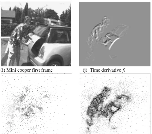
at fourth iteration Fig. 2. A posteriori adaptive optimization process for the determination of optic flow for the marble block image sequenceand the construction of a nice mesh at each step of adaptive process is observed. The plots for various parameters have been presented to show the performance of the given a posteriori optimization process. The numerical results are given in Figure.3.(i-r) below.
(i) Mini cooper first frame (j) Time derivative ft
(k) Flow vector after first adaptation (l) Flow vector after fourth adaptation
(m) Flow Mesh after first adaptation (n) Flow Mesh after fourth adaptation
(o) Flow Magnitude after first adaptation (p) Flow Magnitude after fourth adaptation
[image:4.595.46.293.122.340.2]
(q) Plot of
at first iteration (r) Plot of
at fourth iteration Fig. 3. A posteriori adaptive optimization process for the determination of optic flow for Minicoper image sequence.V. CONCLUSION
A posteriori adaptive strategy introduced in [3, 7] was applied to the nonlinear variational model (3) to refine the initial optimized approximate solution (optic flow) in a posteriori way of optimization process. It was observed that the adaptive procedure presented in this paper improved the quality of initial optimized approximate solution (optic flow) from the nonlinear optimization model (03) at each step of a posteriori local adaptation.
It was shown with simulations for this moving Marble block example that the initial approach of [3] performs even better when the model is improved as nonlinear and thus furnishes a general tool which could be used with many existing models in the literature of computer vision problems. As the method given in this paper is quite new and stills requires some improvements like the settings of the thresholds and other regularization parameters appearing in the given nonlinear model.
The strategy for the given a posteriori adaptation to select the regularization parameter, furnishes a distribution of
which reveals the precise effects of the regularization for an efficient computation of the flow. Moreover the work is interesting should be pursued for various other applications in imaging techniques. The further numerical experiments along with error profiles and comparisons with existing well rated methods are under consideration with more real world images will be performed in near future..
ACKNOWLEDGMENT
“Author is highly thankful to Prof. Zakaria Blehachmi (France), and Prof. F.Hecht (France) for every possible guidance to conduct this work and specially their helps in conducting these experiments. K.B Amur would like to thanks QUEST Nawabshah Pakistan for providing every support during the conduct of this work”.
REFERENCES
[1] M. G. Mozerov and J. van de Weijer, “Accurate stereo matching by two-step energy minimization,” IEEE Transactions on Image Processing, Vol.24, pp. 1153–1163, 2015.
[2] H. W. Engl, M. Hanke, and A. Neubauer. Regularization of inverse problems, volume 375 of Mathematics and its Applications. Kluwer Academic Publishers Group, Dordrecht, 1996.
[3] Belhachmi Z. and F.Hecht, “Control of Effects of the regularization on Variational optic flow computations”. J. Mathematical imaging and vision, VOl. 40, No.1, pp. 1-19, 2011.
[4] J. Abhau, O. Scherzer, Belhachmi Z, “On a Decomposition Model for optical flow and Stereo-Vision Problems,” EMMCVPR 09 Proceedings of the 7th Conference on Energy Minimization Methods in Computer Vision and Pattern Recognition, volume 5681, pages 126-139, Berlin, Heidelberg, 2009. Springer-Verlag.
[5] Tikhonov A. N, “Solution of incorrectly formulated problems and the regularization method,” Soviet Mathematics Doklady, 4, 1035-1038, 1963.
[6] Markus Grasmair, “Locally Adaptive Total Variation Regularization,” SSVM '09 Proceedings of the Second International Conference on Scale Space and Variational Methods in Computer Vision Pages 331-342.
[7] Amur K.B, “Contrôle adaptatif, techniques de régularisation et applications en analyse d’images”. PhD. thesis LMAM University of Metz France, 2011.
[9] Amur K.B, “A Posteriori Control of Regularization for Complementary Image motion Problem,” Sindh Univ. Res. Jour. (Sci. Ser.), vol. 45, no. 3, pp. 546-552, 2013.
[10] Amur K. B, A. L. Memon, and S. Qureshi, “FEM based Approximations for the TV Denoising Optimization Problem,” Mehran University Research Journal of Engineering & Technology, Vol. 33: No. 1, 121-128, 2014.
[11] Horn, B., B. Shunk, “Determining Optical flow,” Artificial Intelligence, Vol.17, 185-203, 1881.
[12] Bruhn A, “Variational Optic Flow Computation, accurate modeling and efficient numerics,” PhD thesis in computer Science Saarbrcken, Germany, Saarland University, 2006.
[13] Zimmer, H. Andres Bruhn, Jaochim Weickert, Levi Valgaerts, Agustin Salgado, Bodo Rosenhahn, and Hans-Peter Seidel, “Complementary optic flow. 7th International Conference, EMMCVPR, Bonn, Germany, 24-27 and Springer, Lecture Notes in Computer Science Volume 5681, pp 207-220, 2009.
[14]Bruhn, A., J. Weickert, Christophschnorr (2005). Lucas/Kanade meets Horn/Schunck: Combining Local and Global Optic flow methods, International Journal of computer vision 61(3), 211-231. [15] Anandan P, “A computational framework and an algorithm for the
measurement of visual motion,” International Journal of Computer Vision, vol. 39, No 01, 41-56, 2000.
[16] Aubert, G., R. Deriche, P. Kornprobst, “Computing optical flow via variational techniques,” SIAM Journal on Applied Math., Vol. 60, NO. 1, pp. 156-182, 1999.
[17] R.B. Ari and N.A. Sochen, “Variational stereo vision with sharp discontinuities and occlusion handling” In the Proceedings of the 2007 IEEE International Conference on Computer Vision, Rio de Janeiro, Brazil, IEEE Computer Society Press. pp. 1–7, 2007. [18] Hecht, F, “New development in FreeFem++”, Journal of Numerical
Mathematics, 3-4, pp .251-265, 2012.