Abstract—The paper deals with an influence of seasonal adjustment of the time series on its time-frequency spectrogram modeling. Because some economic time series is not available in online sources in the seasonal adjusted form, the researchers have to decide whether he use seasonally adjusted or unadjusted data. If they make a seasonal adjustment as a pre-processing of the data, they can use several adjusting methods. We are going to show, how the seasonal adjustment can influence the wavelet modeling of the time series and how it can influence interpretation of the results.
Index Terms— seasonal adjusting, spectrogram, spectrum, wavelets
I. INTRODUCTION
HE wavelet transform is a widely used approach for the time-frequency modelling of input signals or time series. This methodology was successful transferred from engineering to econometrics, where it becomes very popular, especially for its ability to good time resolution. There are several further benefits of the wavelet modelling which attracts economic researchers, namely the use for non-stationary inputs and the ability to uncover complicated patterns over time [1]–[5]. Thus it gives possibility for tracking time and frequency behaviour if the time series simultaneously with good time resolution.
While engineering inputs, e.g. signals, are usually sum of harmonic components with known physical essence, in econometrics the same character and behaviour of inputs, e.g. time series, is different. Economic time series are sum of several cyclical component with more complicated pattern [1]. We can distinguish several regular components in the time series, namely long-term trend component, cyclical movements (long-, medium-, short-cycles) and seasonal movements (i.e. seasonal variations; very short cycles). The last one, a seasonal component, covers fluctuations up to one year. The shape of all these components depends on the nature of the time series. Some cyclical component can occur only for limited time, and in some moment the frequency component can diminish.
Manuscript received March 18, 2019; revised April 03, 2019. The research described in the paper was supported by the Czech Ministry of Education in the frame of National Sustainability Program under grant LO1401. For research, the infrastructure of the SIX Center was used.
Jitka Poměnková is with the FEEC DREL, Brno University of Technology, Technická 10, 616 00 Brno, Czech Republic (e-mail: [email protected]).
Eva Klejmová is with the FEEC DREL, Brno University of Technology, Technická 10, 616 00 Brno, Czech Republic (e-mail: xklejm00@stud. feec.vutbr.cz).
Before the researcher begun with econometric analysis, he have to decide whether he use seasonally adjusted or unadjusted data. The decision which type of data will be used depends on the several factors: the aim of the research, the data consensus in given application area (business cycle analysis, financial cycle analysis etc.) or the assumptions of methodology instruments. The motivation for seasonal adjustment (SA) we can find in the need of standardizing socioeconomic series to get comparable results, because the seasonality can influence an economic indicators in a different way (different intensity, time duration, etc.). If we decide for SA we have to keep on mind the methodological aspect and consequences, which adjusting can brings/takes. In some econometric analyses (VAR modelling, cointegration analysis or business cycle analysis [6] is required a seasonal adjusted time series. Application of wavelets is possible for both, seasonal adjusted as well as seasonal unadjusted (NSA) time series. With respect to the different character of inputs, the results of wavelet analysis have to be carefully interpreted especially in econometric applications.
We are going to show how the seasonal adjusting can influence the result of wavelet modeling compare to the wavelets transform of unadjusted time series. Further, we show that different adjusting methods can produce different adjusted time series, i.e. different wavelet transform, which can remove other components than only a seasonal component and further, seasonal and other cyclical components can interact. These findings show possible impact of SA on economic interpretation of achieved results. And thus we stress an importance of the aim of the analyses’ research in the decision of the type of the data.
For the demonstration of SA influence, and in order to identify the cyclical behaviour of the financial data, we use the seasonally unadjusted real monthly data of bank loans provided to corporates (Corporates) and households (Households) in the Euro Area in 2000/M1–2017/M05.
II.WHAT CAN HELP US TO DECIDE BETWEEN SA AND NSA We want to analyses the cyclical behavior of bank loans activities provided to corporates and households via time-frequency wavelets, because the wavelets has very good ability to describe time-frequency character of cyclical behavior contrary to the time domain or frequency domain techniques. The wavelets can be applied on both SA and NSA data; therefore we have to decide which type of data we use. If an analyst is focused on the description of the
An Influence of a Seasonal Adjustment on the
Time-Frequency Wavelet Modelling of a Bank
Loans Activities
J. Poměnková, E. Klejmova
cyclical behavior of economic inputs such in our case, then there are several reasons, economic as well as methodological, to analyze unadjusted series rather than adjusted time series.
Firstly, our economic data is usually the time series representing behavior of some economic subjects, which can brings information important for consumption and investment activity. Therefore we are also interested in the seasonal character of the data, because it is a part of its cyclical behavior. Thus, information about a cyclical character, including seasonal behaviour, is valuable because the analysis of unadjusted data: i) better reflects the real behavior of subjects which can be influenced by seasonality; ii) it can bring more valuable information to policy makers than adjusted data, which can lead to more efficient monetary policy and more efficient application of instruments of monetary policy. Therefore, it is appropriate to keep the seasonal component of times series in the data. It is good for the policy makers to know if households and corporations react to seasonality as part of the cyclical behaviour and to which extent, because then they can use policy instruments to arrange this reaction or to mitigate the impact on the economic cycle which is influenced by loans. The use of adjusted time series may lead to losing some information, which can reduce the efficiency of monetary policy and limit the achievement of objectives. Thus, it is worth leaving, from economic point of view, the seasonal effect in the data. The analysis of adjusted data is also possible and can bring valuable information, but then the researcher’ interest should be properly specified keeping on mind methodological aspects of adjusting.
The second reason for using seasonally unadjusted data is methodological. The seasonal effect is usually expected in cycles up to one year (very short cycles). As the literature says [7]–[10]: (i) the seasonal component is not independent of the cyclical component; (ii) the character of the seasonal component can change in time and depends on the nature of the series; (iii) “the evaluation of the seasonal component provided by an adjustment method is hampered by the fact that the true seasonal component remains a theoretical and imprecise concept, never liable to direct observation”; (iv) “then, the objectives of seasonal adjustment appear multiple and implicit: Is it to obtain the best estimate of the trend-cycle component or the best estimate of the seasonal component itself or even a prediction of the next months or next year? Each objective will generate its own quality criteria”; (v) “finally; the expected content of a quality report usually differs according to the user. Producers, database managers, analysts, researchers, and policy makers do not need and do not look for the same kind of information”. That is, different adjusting methods can produce different adjusted time series which can remove other components than only a seasonal component, and seasonal and other cyclical components can interact.
There are some authors who use unadjusted data for bank loans analysis [8]–[10]. Namely [8] use credit-to-GDP ratio from BIS statistics, and measure the financial cycle length using quarterly data via wavelets [8] in the case of developed and emerging economies. Both ECB and BIS statistics produce credit data which is not seasonally
adjusted; while BIS produces quarterly data, ECB produces monthly data.
They are also some authors who work with seasonally adjusted data [11],[12] as well as unadjusted data [8]–[10]. However, the authors who use adjusted methods use such methods (different from the method of time-frequency wavelets) of credit cycles’ identification (e.g. VAR models) that require seasonal adjustment. Some authors who use unadjusted methods use wavelets for modelling [8], or they use several methods including wavelets [10],[13]. Galati et al. [9] did not provide a proper specification of all data and the transform used probably because they take the seasonal component as part of cyclical component (short- to medium-term cycles) to achieve their aim. [10],[13] or Rünstler et al. [13] use several unadjusted time series and mention the use of annual growth rates for wavelets to eliminate cycles at annual frequencies as they expect a suppression of seasonal component. But these papers do not include additional information, as provided by Mazzi et al. [7], about the influence of adjusting on finite data. Probably it is because the proper adjusting (the quality of seasonal component suppression) does not have an impact on the paper goal.
Generally, in the case of monthly data we can expect that the seasonal component will range in frequencies up to 12 months. Since wavelets can model the time-frequency behaviour of time series, we can assume that the wavelet spectrogram in the range of 2 months to approximately 12-month length cycles (i.e. short-run cycles in our paper) can contain, in the case of seasonally unadjusted time series, seasonal as well as cyclical components.
III. METHODOLOGY A.Seasonality
Seasonality is caused by the fact that some months/quarters are more important in the level of an analysed economic indicator during the year. Or, some months/quarters are important for some economic activity. The seasonality measures the relative importance of the months/quarters of the year. The idea of seasonal adjustment is to remove seasonal variations in the original time series (i.e. economic indicator) jointly with trading day variations and moving holiday effects [7].
B.Seasonal Adjustment Methods
There are several different seasonal adjustment methods. In our paper we are going to investigate:
X-11-ARIMA: proposed by Dagum [14] at Statistics Canada. It also belongs to the non-parametric smoothing methods based on iterative application of moving averages filters.
TRAMO-SEATS [15]: Time Series Regression with ARIMA Noise, Missing Observations and Outliers (TRAMO) and Signal Extraction in ARIMA Time Series (SEATS) have been developed by Maravall and Gómez [16] and Gómez and Maravall [16][17] at the Bank of Spain [18].
The TRAMO-SEATS consists from two parts. The TRAMO part is designed to remove deterministic effects and make the series stationary. It is based on a mix model consisting of regression variables with ARIMA errors. The SEATS part consists and provides steps leading to the stationarity of the time series via differences of a finite order. X11-ARIMA use an ARIMA (AutoRegressive Integrated Moving Average) model based on the work of Box and Jenkins [19] to time series forecast and backcast before we start with the data processing in order to replace the missing data which results and to make possible use of less asymmetric filters. The original X-11 only arbitrarily extrapolated the missing values. The model integrated in X11-ARIMA use linear filters of the X-11 method which is based on different kinds of weighted symmetric and asymmetric moving averages combined with ARIMA-model filters which are adjusted globally to the data. For the detail specification of both approaches see Mazzi et al. [7].
X13 SEATS is developed by U. S. Census Bureau [20] as an extended and improved version of the X11-ARIMA. The method is based on iterative application of moving averages filters and gives the possibility to apply methods based on an ARIMA model.
C.Wavelet Transform
The wavelet transform can be used for the description of the cyclical movements of the time series in time-frequency domain. The continuous wavelet transform (CWT) can be described as the integral of analysed time series x(t) with the base function (mother wavelet) [22]:
1
( , ) ( ) , 0,
x
t b
W a b x t dt a b R
a
a
(1)where a is the time position, b is the parameter of dilatation (scale) of the mother wavelet
. To satisfy assumptions for the time-scale analysis, waves must be compact in time and frequency representation as well.The Torrence and Compo [23] (TC98) proposed the significance test for the wavelets spectra with the Morlet mother wavelet. The distribution for the local wavelet power spectrum
|
W a b
x( , ) |
2 with the use of Morlet wavelet is2
2 2 2
| ( , ) | 1
~ ,
2
x
k
W a b
P
(2) where the
P
kis the mean spectrum at the Fourier frequency k that corresponds to the wavelet scale a. When the background spectrum is the Gaussian white noise (common for an economic data), theP
k=1.IV. DATA AND SETTINGS A.Data Description
In order to identify the cyclical behaviour, we use the seasonally unadjusted real monthly data of bank loans provided to corporates (Corporates) and households (Households) in the Euro Area in 2000/M1–2017/M05 (Millions of Euros) [21]. Both time series had a length of 209 points. As proved by relevant empirical studies, the wavelet methodology is applicable for cyclical behaviour description of our date range (see [1]–[3],[8]–[10],[24]).
B.Settings
For the seasonal adjustment we applied TRAMO-SEATS, X-11-ARIMA and X13 SEATS methods on both time series, i.e. on Households and Corporates, in MATLAB X-13 Toolbox, Version 1.33[24].
To obtain primary evaluation of the methods, we transformed the SA time series into the frequency domain using Welch's power spectral density estimate [26]. Based on the length of the data we used Hamming window with 50% overlap and 128 discrete frequency points.
To get more complex results in the time-frequency domain we used CWT. We set the scales to correspond the range of 0.5 year to 10 years with 334 individual scales. This range was chosen to be consistent with standard econometric modelling. We selected Complex Morlet wavelet with center frequency fb=1.5. For the significant testing we use TC98
approach on resulting CWT spectrograms; the significance level is α=0.05.
V.RESULTS
An empirical analysis proceeds in following steps: i) we perform the CWT of each NSA series to obtain the spectrograms; we use the significance testing via TC98; ii) we apply methods for seasonal adjusting, namely TRAMO SEATS, X12 ARIMA and X 13 SEATS ; iii) consequently we estimate corresponding spectra via Welch's periodogram for each SA time series of households and corporates; iv) we perform the CWT of each SA series to obtain the spectrograms; iv) we compare and discuss the achieved results.
To make the orientation in the spectrogram figures and the description of the results easier, we are going to divide the cyclical behavior into the following regions: the very short cycles of duration <12 months, the short cycles of duration 12–20 months, the medium cycles of duration 20– 48 months and the long cycles over the 48 months. Denote that the wavelet spectrogram in the very short cycles can contains seasonal and some cyclical component.
A.Wavelet Transform for Seasonal Unadjusted Data
In the first step of an empirical analysis we use seasonally unadjusted data. Their wavelet transform is displayed in Fig. 4 a-b). In the case of Corporates the significant part of spectrogram, i.e. the significant time-frequency regions, can be visible for medium and long cycles, and in very short cycles. The detail description proposes Table I.
B.Spectra
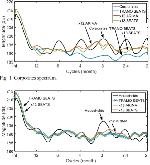
In the next step we apply methods for seasonal adjusting, namely TRAMO SEATS, X12 ARIMA and X 13 SEATS. After adjusting we estimate corresponding spectra via Welch's periodogram for each SA time series of households and corporates. The resultant comparisons of spectra are proposed in Fig. 1–2.
adjusting methods. The spectra estimates differ just with unadjusted time series.
[image:4.595.318.548.348.758.2]Fig. 1. Corporates spectrum.
Fig. 2. Households spectrum.
C.Wavelet Transform for Seasonal Adjusted Data
As the following step of our empirical analyses we perform the CWT of each SA series to obtain the wavelet spectrograms. Resultant figures are displayed in Fig. 3c-h. In both, Corporates and Households, and all type of seasonal adjustment the significant part of wavelet spectrogram (the significant time-frequency regions) covers all types of cycles (i.e. very short cycles, medium and long cycles). The detail description proposes Table I.
D.Comparison of Results Achieved by SA and NSA
In the last step we focus on comparison of archived results (Fig. 2 and in Tabular I). Firstly we focus on frequency range of very short cycles which covers fluctuations up to one year including seasonal component. In case of Corporates the spectrogram for SNA data indicates such fluctuations only till the 2009. The seasonal adjustment reveal, that seasonal component interact with other very short fluctuations, because after adjusting we still identify some significant regions. Focusing on the different adjusting method we realised different results, especially after 2009 were the significant region is smaller or bigger depending on adjusting method. In case of Household all adjusting methods produce generally same very short cycles. Compare to the spectrogram for NSA data we identify additional significant area in 2013-2014 and we did not identify cycles before 2007. That is, adjusting suppress some very short cycles and reveal additional very short cycles after 2013. The main finding from the economic point of view is that seasonal component is time changing which confirmed all the spectrogram figures.
In other frequency ranges, i.e. the short, medium and long cycles, the results for Households and Corporates are
different. In the case of Household, all three adjusting method produce time series which after wavelet spectrogram modelling show generally same results. Comparing Households for SA and SNA spectrograms we can see that adjusting highlighted the short and the medium cycles. In the case of Corporates the results for the short and medium cycles are different. Only in the case of the long cycles we can see similarity among adjusting methods. Firstly, adjusting highlighted cyclicality in the short cycles with a different amplitude depending on adjusted method. Secondly, adjusting highlighted and spread the cyclicality in the medium cycles. To summing up results for Corporates we can see that adjusting suppressed some components, it revealed additional components (in short cycles) and highlighted and spread medium cycles.
The main finding from the economic point of view is, that seasonal and other cyclical components interact and that they are cases where different adjusting methods can produce a different adjusted time series with a different cyclical structure. Such finding can have an important impact on an economic interpretation.
TABLEI
SIGNIFICANT AREA OF WAVELET SPECTROGRAM OVER
FREQUENCY INTERVALS
Very short cycles (<12 months)
Short cycles (12-20 months)
Medium cycles (20–48 months)
Corporates; NSA 2001/Q1-2002/Q3
2003/Q3-2009/Q1 -- 2004/Q3-2015/Q1 Corporates; SA: TRAMO-SEATS
2000/Q1-2001/Q2 2004/Q2-2008/Q4 2011/Q1-2013/Q3
2006/Q3-2013/Q3 2004/Q4-2015/Q3
Corporates; SA: X 12 ARIMA
2005/Q4-2008/Q2
2011/Q2-2013/Q3 2011/Q2-2013/Q3 2004/Q4-2016/Q2
Corporates; SA: X 13 SEATS
2004/Q3-2008/Q2
2011/Q3-2012/Q3 2008/Q1-2010/Q1 2004/Q1-2016/Q1
Households; NSA
2000/Q4-2002/Q2 2004/Q4-2007/Q1 2008/Q2-2013/Q1 2014/Q2-2016/Q1
2007/Q1-2012/Q2 2006/Q1-2016/Q3
Households; SA: TRAMO SEATS
2007/Q3-2009/Q3
2013/Q3-2014/Q4 2007/Q3-2014/Q4 2006/Q1-2016/Q3
Households; SA: X 12 ARIMA
2007/Q3-2009/Q3
2013/Q3-2014/Q4 2007/Q3-2014/Q4 2006/Q1-2016/Q3 Households; SA: X 13 SEATS
2007/Q3-2009/Q3
a) Corporates b) Households
c) Corporates X12 ARIMA d) Households X12 ARIMA
e) Corporates TRAMO SEATS f) Households TRAMO SEATS
g) Corporates X13 SEATS h) Households X13 SEATS
[image:5.595.88.512.46.739.2]VI. CONCLUSION
The paper deals with an analysis of an influence of the seasonal adjustment on the time-frequency modeling on a time series. We showed that the seasonal adjusting can influence the cyclical character of a time series in wide range of cycles, i.e. in the very short, the short and the medium cycles. Moreover, we confirmed an interaction of both the cyclical and the seasonal components in the frequency range 6–12 month, and changes of the seasonal component during the time. Furthermore, we showed that the different adjusting methods can produce the different adjusted time series (the different wavelet transform) which can remove other components than only a seasonal component and further, seasonal and other cyclical components can interact. These findings show possible impact of a seasonal adjustment on an economic interpretation of achieved results. And thus we stress an importance of the aim of the analyses’ research in the decision of the type of the data. Therefore, to keep the comparability of the results it is suitable to investigate the influence of data.
REFERENCES
[1] Ch. Aloui, B. Hkiri, D. K. Nguzen, “Real growth co-movements and business cycle synchronization in the GCC countries: Evidence from time-frequency analysis, ” Economic Modeling, vol. 52, pp. 322-331, 2016.
[2] Z. Ftiti, A. Tiwari and A. Belanés, “Tests of financial market contagion: Evolutionary cospectral analysis v.s. wavelet analysis,”
Computational Economics, vol. 46, n. 4, pp. 575–611, 2014.
[3] A. N. Berdiev and Ch.-P. Chang, “Business cycle synchronization in Asia-Pacific: New evidence from wavelet analysis,” Journal of Asia
Economics, vol. 37, pp. 20–33, 2015.
[4] A. K. Tiwari, M. I. Mutascuand C. T. Albulescu, “Continuous wavelet transform and rolling correlation of European Stock markets,” International Review of Economics and Finance, vol. 42, pp. 237–256, 2016.
[5] L. Aquiar-Conraria and M. J. Soares, “The Continuous Wavelet Transform: moving beyond uni and bivariate analysis,” Journal of
Economic Survey, vol. 28, n. 2, pp. 344–375, 2014.
[6] W. H. Green, Econometric analysis, 7th~ed. Prentice Hall, 2012. [7] Mazzi et al., Handbook on Seasonal Adjustment, Luxembourg:
Publications Office of the European Union, 2018.
[8] M. Altar, M. Kubinschi and D. Barnea, “Measuring financial cycle length and assessing synchronization using wavelets,” Romainan
Journal for Economic Forecasting, vol. 20, n. 3, pp. 18–36, 2017.
[9] G. Galati, I. Hindrayanto, S. J. Koopman and M. Vlekke, “Measuring financial cycles in a model-based analysis: Empirical evidence for the United States and the euro area,” Economic Letters, vol. 145(C), pp. 83–87. 2016.
[10] D. Kunovac, M. Mandler and M. Scharnagl, “Financial cycles in euro area economies: A cross-country perspective,” Discussion Papers
04/2018, Deutsche Bundesbank, 2018.
[11] T. Helbling, R. Huidrom, M.A. Kose and C. Otrok, “Do credit shocks matter? A global perspective,” European Economic Review, vol. 55, no. 3, pp. 340–353, 2011.
[12] V. Ivashina and D. Scharfstein, “Bank lending during the financial crisis of 2008,” Journal of Financial Economics, vol. 97, n. 3, pp. 319–338, 2010.
[13] G. Rünstler, H. Balfoussia, L. Burlon, et al, “Real and financial cycles in EU countries - Stylised facts and modelling implications,”
Occasional Paper Series 205, European Central Bank, 2018.
[14] E.B. Dagum, “The X11ARIMA seasonal adjustment method,” Statistics Canada, Ottawa, Canada, Catalogue No. 12-564, 1980. [15] V. Gómez and A. Maravall, “Programs Tramo and Seats: Instructions
for the User,” Beta version, Banco de Espaňa, 1997.
[16] A. Maravall and V. Gómez, “Signal extraction in ARIMA time series: Program SEATS,” Working Paper ECO No 92-65, Department of Economics, European University Institute, 1992.
[17] V. Gómez and A. Maravall, “Programs TRAMO and SEATS: Instructions for the user (beta version: June 1997),” Working Paper No 97001, Dirección General de Anélisis y Programación Presupuestaria, Ministerio de Economía y Hacienda, Madrid, 1997. [18] A. Maravall and G. Caporello, “Program TSW: Revised reference
manual. Technical Report,” Research Department, Bank of Spain, 2004.
[19] G. E. Box, G. M. Jenkins, G. C. Reinsel and G. M. Ljung, Time series analysis: forecasting and control. John Wiley & Sons. 20115. [20] U. S. Census Bureau. “X12-ARIMA Reference Manual, Beta
Version,” Statistical Research Division, 1997.
[21] ECB (2017). Euro area statistics: Banks balance sheet – loans [online database]. [cit. 2017-09-18]. Retrieved from
https://www.euro-area-statistics.org/banks-balance-sheet-loans?cr=eur
[22] D.~F. Walnut, An introduction to wavelet analysis, Springer Science \& Business Media, 2013.
[23] Ch. Torrence and G. P. Compo, “A practical guide to wavelet analysis,” Bulletin of the American Meteorological society, vol. 79, no. 1, pp. 61–78, 1998.
[24] J. Fidrmuc, I. Korhonen and J. Poměnková, “Wavelet spectrum analysis of business cycles of China and G7 countries,” Applied
Economic Letters, vol. 21, no. 18, pp. 1309-1313, 2014.
[25] Y. Lengwiler, “X-13 Toolbox for Matlab, Version 1.33,” Mathworks
File 2017,
http://ch.mathworks.com/matlabcentral/fileexchange/49120-x-13-toolbox-for-seasonal-filtering
[26] J. G. Proakis, C. M. Rader, F. L. Ling, et al, Algorithms for statistical