Uses of the pitch scaled harmonic filter in speech processing

USES OF THE PITCH-SCALED HARMONIC FILTER

IN SPEECH PROCESSING

Philip J.B. Jackson School of Electronic and Electrical Engineering, University of Birmingham, Edgbaston, Birmingham B15 2TT, UK. [[email protected]]

Christine H. Shadle Department of Electronics and Computer Science, University of Southampton, Highfield, Southampton SO17 1BJ, UK. [[email protected]]

Abstract

The pitch-scaled harmonic filter (PSHF) is a technique for decomposing speech signals into their periodic and aperiodic constituents, during periods of phonation. In this paper, the use of the PSHF for speech analysis and processing tasks is described. The periodic component can be used as an estimate of the part attributable to voicing, and the aperiodic component can act as an estimate of that attributable to turbulence noise, i.e., from fricative, aspiration and plosive sources. Here we present the algorithm for separating the periodic and aperiodic components from the pitch-scaled Fourier transform of a short section of speech, and show how to derive signals suitable for time-series analysis and for spectral analysis. These components can then be processed in a manner appropriate to their source type, for instance, extracting zeros as well as poles from the aperiodic spectral envelope. A summary of tests on synthetic speech-like signals demonstrates the robust-ness of the PSHF’s performance to perturbations from additive noise, jitter and shimmer. Examples are given of speech analysed in various ways: power spectrum, short-time power and short-time harmonics-to-noise ratio, linear prediction and mel-frequency cepstral coefficients. Besides being valuable for speech production and perception studies, the latter two analyses show potential for incorporation into speech coding and speech recognition systems. Further uses of the PSHF are revealing normally-obscured acoustic features, exploring interactions of turbulence-noise sources with voicing, and pre-processing speech to enhance subsequent operations.

1

Introduction

2

Method

Our decomposition technique, the PSHF, is based on a measure of harmonics-to-noise ratio derived by Muta et al. [8]. Calculating the HNR from a short section of speech

, they used the tral properties of an analysis frame scaled to the pitch period for distinguishing parts of the spec-trum containing periodic energy from those without. Using a four pitch-period Hann window,

for

, centred at time , they windowed

to form !

#"

$%

, where the length&

!(')*

was a whole number of pitch periods)+*

(in sam-ples,

',(-). The spectrum. !/

was calculated by DFT, which concentrated the periodic part of into the set of harmonic bins,0

'

' 1

'

' 2(

. Here, the harmonics are translated to bins

3

. The value

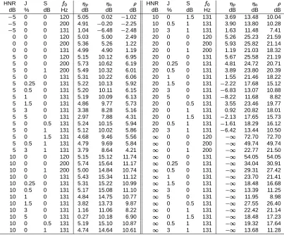
'(-was used because four is the smallest number that leaves bins free of spectral leakage from the periodic component (those half-way between the harmonics:

4

), as shown in Figure 1. A larger value of'

would make the decomposition more susceptible to degra-dation from the many kinds of variation in speech, e.g., in amplitude, fundamental frequency, formant frequencies, at voice onset/offset).5 So, for speech with a pitch period of 6 ms and

'

= 4, the window would be 24 ms long.

−7 −6 −5 −4 −3 −2 −1 0 1 2 3 4 5 6 7

−80 −60 −40 −20 0

Normalised frequency (bins)

Amplitude (dB)

Figure 1: Comparison of the smearing effects on the spectral envelope of rectangular (solid) and Hann (dashed) windows.

The gain in robustness from using a Hann window, compared to a rectangular window, can be de-scribed by the sensitivity of cross-term bias errors between harmonics to deviations from perfect peri-odicity. These errors are reduced by a factor of 15 by the Hann window at the adjacent harmonic, four bins away. Also, the half-power bandwidth of the main peak at each harmonic is increased by 60 %, though it is related to an increase in estimation variance. In summary, a small part of the maximum likelihood performance for perfectly periodic signals is compromised to make the PSHF more suitable for time-varying signals.

While windowing allows the piecewise-stationary PSHF to adapt, we need to recombine the output signals after decomposition, which is achieved by overlapping and adding. However, we also need to normalise the aggregate back to unity gain, using the factor

6

!

798 :

8

8

"&&

8

;

(1)

<

where the summation includes all windows=>, centred at?+>, that contain time? . A cosine ramp was applied to each end of the normalisation factor@ABC to fade out sections of voicing at onset and offset.

We have extended the process to yield a full decomposition into periodic (estimate of voiced) and aperiodic (estimate of unvoiced) complex spectra, which can be converted back into time series D

E

and D

F

respectively by inverse Fourier transformation and windowing, as explained below. We have also proposed an interpolation step for improving power-spectral estimation, which producesG

E

andG

F

[5, 7]. The signals can later be analysed using any standard technique (as will be demonstrated later in this paper): D

E

and D

F

for time-domain analysis, G

E

and G

F

for frequency-domain analysis. For time-frequency analysis, we define a threshold frame size of half the mean PSHF window length, HIJ K L or two pitch periods, which is the point at which the harmonics begin to be resolved. Thus, D

E

and D

F

would be used for wide-band spectrograms, and G

E

and G

F

for narrow-band ones.

2.1 Pitch estimation

Requiring that the window lengthI be scaled to the time-varying pitch periodM+N A?+C means that we must first estimate the pitch period of any speech signal. Initial estimates may be obtained manually or from the autocorrelation, for instance. The pitch-estimation algorithm then finds optimum value, for a particular time, by minimising the amount of smearing in the spectrum from the firstO harmonics, PQR S T

L

T U U U T

OV . Thus, the spectral sharpness is expressed in terms of the higher and lower spectral spread,WX

Y and W!Z

Y respectively, as defined in [8], and the cost function is

[

AI

T

?+C!\

]

^

Y _`

a

WX

Y

AI

T

?+C b!cdW!Z

Y

AI

T

?+C b e

T

(2)

providing a pitch estimate perfectly matched to the decomposition, as described below. See [8] for further details. Thus, a pitch track can be obtained by repeating this process at successive points throughout the speech signal.

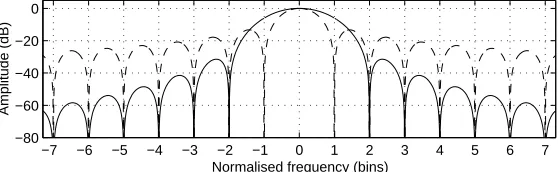
2.2 Algorithm: Harmonic filter

Let us consider how the PSHF decomposes a single frame, centred at time? , in its harmonic filter, the central engine of the algorithm. After applying the pitch-scaled Hann window to the speech signal, f g

ABC is discrete Fourier transformed (DFT) toW

g

Ah C , as depicted byi in Figure 2. The harmonic filter extracts the pitch harmonics fromW

g

, doubling their coefficients to compensate for the mean window amplitude, which form the harmonic spectrum:

D

j

Ah C!\k L W

g

Ah C forh Q$l

m

otherwiseT (3)

wherel

\

R n+To T U U U Tn AIdp

S

V(k)^ S (k)_w

s (n)_w

u (n)_w ^ v (n)_w ^ s(n) window q harmonic filter + -q -1 window

Figure 2: The pitch-scaled harmonic filter (PSHF) comprising Hann window, discrete Fourier trans-form (r ), harmonic filter, inverse DFT (r$st ) and another Hann window operation to yield the outputs for time-series processing,u

v w and u

xw .

pitch periods are windowed to yield the periodic signal estimate:

u

v w!yz{!|d} yz{ ~€ st  ‚ ƒ„… u †

y‡ { ˆ ‰ Š‹ Œ Ž z‡

~‘’ (4)

The aperiodic signal estimate is the difference between the input signal and the periodic estimate:

u

xwyz{!|9“ w!yz{ ”

u

v wyz{

. This could be obtained equivalently via the frequency domain: u

•

y‡ {!|(–y‡ { ”

u

†

y‡ {

, by IDFT and windowing.— As a result of the subtraction, any errors in the periodic estimate caused by the decomposition algorithm are (wrongly) attributed to the aperiodic signal.

2.3 Algorithm: Power interpolation

The spectrum of the (windowed) aperiodic signal, u

•

wy‡ {

, contains gaps at the pitch harmonics where the coefficients are of zero amplitude, since u

•

w!y‡ {#|˜–w!y‡ {!”

u

†

w!y‡ {#|d–w!y‡ {”9y



–wy‡ {{™



|dš for ‡$›$œ

. However, subsequent analysis often involves spectral magnitudes, power spectra or spectro-grams, and so the gaps would give strongly biased under-estimates. We can improve these estimates by patching suitable values into u

•

w

at the harmonics, according to the process shown in Figure 3.

2

λ

1-λ

v (n)_w ~

u (n)_w ~ ^ U(k) V(k) ^ + + ž -1 ž -1 window window

Figure 3: The PSHF’s interpolation stage, which redistributes the power at the pitch harmonics to produce the outputs for spectral processing, the componentsŸ

v w and Ÿ

xw .

Assuming the aperiodic component to be stochastic with a smooth frequency response, the power in any frequency bin‡

is expected to be similar to that of the adjacent bins‡¡ 9¢

. Hence, we calculate

£

Unwindowed spectra,¤¥¦ §, ¨

©

¥¦ § and ¨

ª

¥¦ §, correspond to unwindowed signals in the time domain:« ¥¬ §,

¨

­

¥¬ § and

¨ ® ¥¬ §. ¯ ¨ © °

¥¦ § is half of

¨

©

, a frequency-local estimate ofµ¶· µ at the harmonics, by interpolation of the adjacent powers:

±,²³ ´¸˜¹ º »¼½ ½ ½ ¾ ¶· ²³À¿ º ´ ½ ½ ½Á! ½ ½ ½ ¾ ¶· ²³  º ´ ½ ½

½Á Ã

for³Ä$ŘÆ

(5)

The factorÇ ²³ ´

determines the distribution ofÈ· ²³ ´

’s power between the revised periodic and aperi-odic estimates by comparing it with±²³ ´

’s power, thus:

Ç

²³ ´!¸

±²³ ´

É

µÈ· ²³ ´

µ

Á

Â

²±²³ ´ ´

Á

Æ

(6)

The revised estimates are:

Ê

Ë%²³ ´!¸ÌÎÍ

º

¿

Ç

²³ ´

Á

¾

Ë$²³ ´

for³Ä$Å ;

¾

Ë$²³ ´

otherwise, and

Ê

¶

²³ ´!¸Ì

¾

¶

²³ ´

Â

Ç

²³ ´

¾

Ë$²³ ´

for³Ä$Å ;

¾

¶

²³ ´

otherwise. (7) Note that using the original phase information for both components,Ï Ð Ñ

²

È· ²³ ´ ´

, enables us to re-construct the power-based time series Ê

Ò · ²Ó´ and Ê Ô · ²Ó´

(by IDFT and windowing, as before), so that consistency is maintained across overlapping frames. These signals retain the detail of the original time series, while avoiding artefactual troughs at pitch harmonics in the magnitude spectrum. Each of the four outputs,

¾ Ò · , ¾ Ô · , Ê Ò · and Ê Ô

· , can be overlapped with outputs from neighbouring frames to yield two pairs of contiguous periodic and aperiodic components:

¾

Ò

and

¾

Ô

, and Ê

Ò

and Ê

Ô

.

3

Evaluation

The performance of the PSHF was evaluated using speech-like test signalsÕ ²Ó´

, which were made up of a synthetic voiced partÒ

²Ó´

and unvoiced partÔ ²Ó´ : Õ ²Ó´¸ Ò ²Ó´ Â Ô ²Ó´

. The sampling rate was Ö ×

= 48 kHz. The voiced part was produced by convolving a periodic pulse trainØ ²Ó´

with an appropri-ate impulse-response filterÙ

²Ó´ :Ò

¸

Ø!ÚÙ . The filterÙ was built using the linear prediction coefficients (LPC, 50-pole, autocorrelation) obtained from a recorded adult male [aa] vowel. For jitter and shimmer tests, the pulses were randomly perturbed from their nominal amplitude and pitch period by amounts ranging from 0 to 5 % and 0 to 1.5 dB, respectively [4]. The unvoiced part was similarly created by convolving Gaussian white noise Û

²Ó´

(zero mean, unit variance) with the LPC filter: Ô ¸ÎÜ

Û$Ú¡Ù , and the gainÜ

was adjusted to give the desired HNR (¿

5 toÝ dB). Tests using modulated noise are reported elsewhere [5, 6].

So, using the PSHF component estimates

¾

Ò

and

¾

Ô

, the changes in signal-to-error ratio (SER) were calculated, as a measure of the decomposition algorithm’s performance. The change in SER for the periodic componentÞ ß is defined as the ratio of the unvoiced part’s mean power to that of the residual error, à ¸á² ¾ Ò ¿ Ò ´&¸á¿&² ¾ Ô ¿ Ô ´

; conversely, the aperiodic performance Þ â is the ratio of voiced to residual-error power (expressed in dB):

Þ ß

¸

º ãäå Ñ æç¡èé

Ô

Á ê ë éà

Á êìÀí

and Þ â

¸

º ãäå Ñ æç#èé

Ò

Á ê ë éà

Á êì

Æ

(8)

Similarly, we define an estimate of the HNR as:î

¸

º ãäå Ñ æç#èé

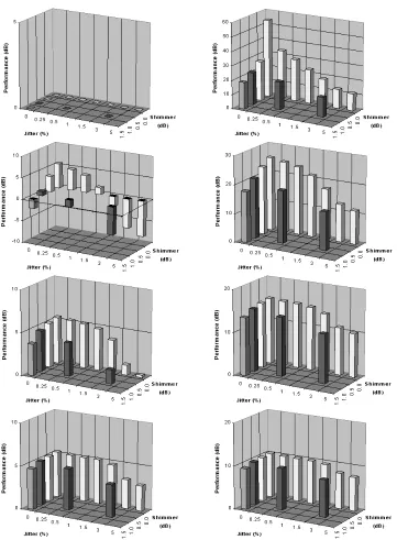
Figure 4: Performance of PSHF for the periodic (left) and aperiodic (right) components,ï ð andï ñ respectively (with no jitter or shimmer). Results are shown here for three values of ò ó (120.0 Hz, 130.8 Hz, 200.0 Hz), and five values of initial HNR (ô 5 dB, 0 dB, 5 dB, 10 dB and 20 dB).

3.1 Test results

Figure 4 shows the effects of the initial HNR and fundamental frequency on performance. For all but one extreme exception (ô 5 dB,ò ó = 130 Hz), the fundamental frequency has a negligible influence, because the resolution of the harmonic filter is effectively constant relative toò ó . For the periodic com-ponent, the effect of HNR is marginal, though it degrades slightly under very noisy conditions, while the aperiodic performance is very dependent on the initial HNR. The results show that the PSHF enhanced the estimate of the voiced component by 5 to 6 dB, and the aperiodic estimate by approxi-mately 5 dB more than the HNR.

With frequency and amplitude perturbations from jitter and shimmer respectively included, there was a similar pattern, albeit increasingly degraded as the degree of perturbation was increased. The re-sults in Figure 5 show that, for perturbation levels normally found in speech, the performances are typically reduced by approximately 1 dB, compare to the unperturbed results. Yet, improvements to the estimate of the voiced part were obtained with severe jitter, shimmer and noise, e.g. (J, S, HNR): (3 %, 1 dB, 5 dB) and (3 %, 0 dB, 10 dB). Fluctuations in the pitch period (jitter) appeared to have a larger effect on the PSHF’s performance than amplitude fluctuations (shimmer).

4

Secondary analyses

An adult male (LJ), a native speaker of European Portuguese, recorded a speech corpus that included sustained fricatives in the form /VF:/ (V = /ax/, F = /v, z, zh/). The sound pressure at 1 m was measured in a sound-treated booth using a microphone (B & K 4165), a pre-amplifier (B & K 2639) and ampli-fier (B & K 2636, 22 Hz to 22 kHz band-pass, linear filter). It was recorded on DAT (Sony TCD-D7, þ ÿ

= 48 kHz), and thence transferred digitally to computer. These speech signals were decomposed by the PSHF in preparation for the subsequent analyses described in the remainder of this section.

0 100 200 300 400 500 600 700 800 900 1000

−0.05 0 0.05 −0.2 0 0.2 −0.2 0 0.2

Time (ms)

Sound pressure

Figure 6: Time series from [ax-v:] by an adult male (LJ) of the original signal

(top), the peri-odic component

(middle), and the aperiodic component

(bottom, note quadruple amplitude scale).

4.1 Time series

Figure 6 illustrates the result of applying the PSHF to part of the utterance [ax-v:]. The voice onset occurred at = 100 ms and the fricative continued until = 5.1 s. The majority of the signal energy is modelled by the periodic component

, which begins mid-vowel during voicing, and is maintained at a high level throughout the vowel. After 100 ms, it starts to fade as the transition is made into the fricative, which overshoots and reaches a steady state at c. 320 ms. In contrast, the noisy aperiodic component

is of a much lower amplitude in the vowel (magnified four times in the graph), decaying to its minimum towards the end of the vowel (c. 150 ms); the frication noise then develops up to 260 ms. As voicing returns in the sustained fricative (c. 280 ms), there are some transient errors manifested as glitches at the pitch epochs. A very low-frequency component is perhaps evidence of flutter (combined effects of jitter and shimmer) that gradually dies away, particularly after 700 ms. However, the high-frequency frication noise continues to arrive in pitch-synchronous pulses. The waveforms show how the noise has been removed from the periodic part

; the noise appears in the aperiodic part

as pitch-synchronous packets.

0 100 200 300 400 500 600 700 800 900 1000 40

50 60 70

Time (ms)

STP (dB)

Figure 7: Short-time powers of the periodic (upper) and aperiodic (lower) components, and , during [ax-v:] by LJ. The dashed lines show short-term variations within each pitch period ( 7 ms, Hann window); the solid lines medium-term ( 30 ms, Hann window).

4.2 Short-time power

The short-time power (STP) is a quantity derived by calculating a moving, weighted average of the squared signal. It is defined, for any signal , as:

!

"$#&%(') *(+ ,-*/.01 2 + 3 4!

"#%65) *7

+ 8 9

(9)

using a smoothing window) *7 , which was set to a fixed length. The STP can be used to examine the pulsing of the noise component, as in [6], but if one is interested in medium-term effects (i.e., at a similar rate to articulatory movements) the oscillation can be removed by averaging over a few pitch periods. This point is illustrated in Figure 7 where the short-term STP (:<;=(>, where; > denotes the time-average) and medium-term STP (?A@&;=(>) are plotted. The STP of the periodic compo-nent, , and that of the aperiodic component, , were calculated using B

C

and B

D

respectively. While confirming our earlier observations, these trajectories provide a clear picture of the timing and rela-tive amplitudes of the different acoustic contributions. Even for this weak fricarela-tive, the aperiodic STP shows a doubling of the noise amplitude on average following the vowel-fricative transition. The differ-ence between the periodic and aperiodic STP curves gives a measure of the short-time HNR, which could be used as an objective means to determine the start of the fricative (e.g., for coarticulation studies).

4.3 Power spectra with linear predictive smoothing

Power spectra were calculated from a steady section of the speech signal and the power-based sig-nals (E ,F

C

andF

D

, centred on 900 ms in Figs. 6/7), and are plotted in Figure 8 (upper half). Most of the energy in the original spectrum comes in the first four harmonics (ofG

%

0 1 2 3 4 40

60 80 40 60 80 100 60 80 100

Frequency (kHz)

0 1 2 3 4 5 6 7 8

40 60 80 40 60 80 100 60 80 100

Frequency (kHz)

PSD (dB/Hz)

0 1 2 3 4

40 60 80 40 60 80 100 60 80 100

Frequency (kHz)

0 1 2 3 4 5 6 7 8

40 60 80 40 60 80 100 60 80 100

Frequency (kHz)

PSD (dB/Hz)

Figure 8: Power spectral density (85 ms, Hann window centred at 900 ms,HI zero-padded, averaged over 170 ms) computed mid-phone for the sustained fricatives by an adult male subject (LJ), (upper) [v:] and (lower) [zh:], using: (top) the original signalJ KLM, (middle) the periodic estimate N

O

KLM and (bottom) the aperiodic estimate N

P

the aperiodic spectrum, being pervasively noisy, is almost completely devoid of harmonics. On the left, smoothed spectra derived from the linear prediction coefficients (50-pole, autocorrelation [1]) are superimposed. They demonstrate how both components differ from the original, in terms of spectral tilt and the frequency and bandwidth of the spectral peaks, e.g., in kHz: original (0.15, 1.38, 2.61), periodic (0.15, 1.34, 2.65), aperiodic (absent, 1.48, 2.61). For comparison, we refer to the peaks as F0, F2 and F3 respectively, and the less-prominent hump near the third harmonic (c. 420 Hz) as F1. Note that the periodic and aperiodic LPC spectra first transect just above 2 kHz because of their tilts, a lower frequency than might be expected.

Figure 8 (lower half) shows the fricative [zh:] uttered by the same subject, having been processed sim-ilarly. Its LPC spectra (left) transect lower still at c. 1.3 kHz as the frication noise dominates from F2 up-wards (see also [z:] by PJ [7]). Peak frequencies (F0, F2, F3) in kHz are: original (0.14, (2.02), 2.57), periodic (0.15, -, 2.49), aperiodic (-, 1.74, 2.44). The bandwidths also differ considerably (cf. F3), and formants are both inserted and deleted with respect to the original.

4.4 Mel-frequency cepstral smoothing

Mel-frequency cepstral coefficients (MFCCs) were calculated according to standard procedures [10]. The binning process used an array ofQ = 26 band-pass filters that were triangular and equally-spaced between 0 and 4 kHz on the Mel-frequency scale:

R

Mel SUT T V WXY[ZT\

R

Hz] W ^ ^ _a` (10)

whereXY implies the natural logarithm. This yields a value for the Mel-frequency log-magnitude spec-trum,b

Zc&_, at each Mel-frequency binc .

s (n)_w s( )ν

DCT

truncate

ln

IDCT window

w

S (k) | | d e d

binning Mel-scale

s(n) s ( )’ν S ( )’ κ

Figure 9: Calculation of smoothed log spectra via Mel-frequency cepstral coefficients (MFCCs).

As shown in Figure 9, the discrete cosine transform (DCT) is applied tob

Zc&_, to form the MFCCs,

f

Zg _ whereg is the coefficient index [1]. These are truncated, as denoted by prime f h

Zg _ , keeping only thirteen (13) values and setting the remainder equal to zero (the zeroth coefficient is also often discarded), and finally the inverse DCT (IDCT) applied to yieldb

h

Zc&_. The frequency-warping (and non-linear frequency weighting) has been removed for the plots in Figure 8 (right). In summary,

f

Zg _iSkj Zg _

l

V

Qnmaop

q

r st-u

b

Zc&_ v w x$y

ZV c6\zT _ {g

V

Q}|a~(

(11)

b

h

Zc&_iSk€4Z c&_

l

V

Q maop

q

 st-u f h

Zg _ v w x$y

ZV g‚\zT _ {c Q}|a~(

where ƒ „… †‡<ˆŠ‰

‹ Œ for … ‡ ;

Ž

otherwise, and 4„&†‡<ˆŠ‰

‹ Œ for  ‡ ;

Ž

otherwise.

The smoothed spectra on the right-hand side of Figure 8 are derived from Mel-frequency cepstral coef-ficients (MFCCs). Here, the amount of smoothing increases with frequency, but still the three curves are distinct for each example. The original MFCC spectrum has separate peaks near the first har-monic (F0‘ 160 Hz) and the next peak above that (F1‘ 450 Hz), as does the periodic MFCC spec-trum. However, F3 is lower for the periodic component, compared with the original. The aperiodic MFCC spectrum also has a peak at F1 (but not at F0), though rather low in frequency (c. 370 Hz), and again its F2 is higher than the others.

For [zh:], the differences between the aperiodic and the other two MFCC spectra are yet more pro-nounced at low frequencies (’ 500 Hz). The MFCC spectra generally fit better than the LPC ones (again more apparent for [zh:]), especially in the vicinity of spectral troughs. These disparities sug-gest that more radical automatic speech recognition systems that can use different models for different classes of acoustic source (e.g., [2]) may be able to gain a significant advantage by processing these components in parallel.

5

Conclusion

We have presented a signal decomposition technique, its evaluation using synthetic signals, and re-sults from its application to real speech. The PSHF enables separate analyses of periodic and ape-riodic components as estimates of the voiced and unvoiced parts in mixed-source speech. The best decompositions are achieved during sustained phonation, since the PSHF is based on a harmonic model. Although severe jitter and shimmer can induce artefacts in the aperiodic component, the eval-uation indicated consistent improvements over typical conditions. Short-time power, LPC and MFCC analyses showed the potential for modelling of these components individually. Coupled with the ex-amples given, they demonstrate that the PSHF algorithm offers novel forms of feature extraction for speech when turbulence noise and voicing co-occur.

References

[1] J. R. Deller, J. G. Proakis, and J. H. L. Hansen. Discrete-time Processing of Speech Signals. Macmillan, NJ, 1993.

[2] L. Deng and J. Ma. A statistical coarticulatory model for the hidden vocal-tract-resonance dynamics. 4:1499– 1502, 1999.

[3] J. Hardwick, C. D. Yoo, and J. S. Lim. Speech enhancement using the dual excitation speech model. Proc.

IEEE-ICASSP, 2:367–370, 1993.

[4] J. Hillenbrand. A methodological study of perturbation and additive noise in synthetically generated voice signals. J. Speech & Hearing Res., 30:448–461, 1987.

[5] P. J. B. Jackson. Characterisation of plosive, fricative and aspiration components in speech

produc-tion. PhD thesis, Dept. Electronics & Comp. Sci., Univ. of Southampton, Southampton, UK, 2000.

[6] P. J. B. Jackson and C. H. Shadle. Frication noise modulated by voicing, as revealed by pitch-scaled de-composition. J. Acoust. Soc. Am., 108(4):1421–1434, 2000.

[7] P. J. B. Jackson and C. H. Shadle. Performance of the pitch-scaled harmonic filter and applications in speech analysis. Proc. IEEE-ICASSP, Istanbul, 3:1311–1314, 2000.

[8] H. Muta, T. Baer, K. Wagatsuma, T. Muraoka, and H. Fukuda. A pitch-synchronous analysis of hoarseness in running speech. J. Acoust. Soc. Am., 84(4):1292–1301, 1988.

[9] S. Narayanan and A. Alwan. Parametric hybrid source models for voiced and voiceless fricative consonants.

Proc. IEEE-ICASSP, 1:377–380, 1996.

[10] S. J. Young, J. Odell, D. Ollason, V. Valtchev, and P. Woodland. The HTK Book. Cambridge Univ. Tech. Services Ltd., Cambridge, UK, version 2.1 edition, 1995. http://htk.eng.cam.ac.uk/.

HNR J S “ ” • –—• ˜š™ HNR J S “ ” • –›• ˜œ™

dB % dB Hz dB dB dB dB % dB Hz dB dB dB

 5 0 0 120 5.05 0.02  1.02 10 0 1.5 131 3.69 13.48 10.04  5 0 0 200 4.91  0.20  2.25 10 0.5 1 131 3.90 13.80 10.28  5 0 0 131 1.04  6.48  2.48 10 3 1 131 1.63 11.48 7.41

0 0 0 120 5.03 5.00 2.49 20 0 0 120 5.26 25.23 21.59 0 0 0 200 5.36 5.26 1.22 20 0 0 200 5.93 25.82 21.14 0 0 0 131 4.99 4.90 1.19 20 0 1 200 1.19 21.03 18.32 5 0 0 120 5.15 10.12 6.95 20 0 0 131 5.67 25.58 21.19 5 0 0 200 5.73 10.62 6.19 20 0.25 0 131 4.81 24.72 20.71 5 0 1 200 5.49 10.32 6.01 20 0.5 0 131 3.89 23.80 20.39 5 0 0 131 5.31 10.22 6.06 20 1 0 131 1.55 21.46 18.22 5 0.25 0 131 5.22 10.13 5.92 20 1.5 0 131  2.22 17.68 15.12

5 0.5 0 131 5.20 10.11 6.15 20 3 0 131 

6.83 13.07 10.88 5 1 0 131 5.19 10.09 6.13 20 5 0 131  8.22 11.68 8.82

5 1.5 0 131 4.86 9.77 5.73 20 0 0.5 131 3.55 23.46 19.77 5 3 0 131 3.38 8.28 5.16 20 0 1 131 0.92 20.82 18.01 5 5 0 131 2.97 7.88 4.31 20 0 1.5 131  2.13 17.65 15.73

5 0 0.5 131 5.24 10.15 5.94 20 0.5 1 131  1.61 18.29 16.12

5 0 1 131 5.12 10.02 5.86 20 3 1 131  6.42 13.44 10.50

5 0 1.5 131 4.68 9.46 5.56 ž 0 0 120



ž 72.70 72.70

5 0.5 1 131 4.79 9.69 5.84 ž 0 0 200



ž 49.74 49.74

5 3 1 131 3.79 8.64 4.21 ž 0 1 200



ž 22.77 21.50

10 0 0 120 5.15 15.12 11.74 ž 0 0 131



ž 54.05 54.05

10 0 0 200 5.74 15.64 11.17 ž 0.25 0 131



ž 34.04 30.91

10 0 1 200 5.00 14.84 10.74 ž 0.5 0 131



ž 29.31 27.42

10 0 0 131 5.43 15.34 11.12 ž 1 0 131



ž 23.70 21.41

10 0.25 0 131 5.31 15.22 10.99 ž 1.5 0 131



ž 18.48 16.68

10 0.5 0 131 5.17 15.08 11.10 ž 3 0 131



ž 13.39 11.25

10 1 0 131 4.84 14.75 10.77 ž 5 0 131



ž 11.95 8.98

10 1.5 0 131 3.82 13.73 9.87 ž 0 0.5 131



ž 27.55 26.40

10 3 0 131 1.16 11.06 8.22 ž 0 1 131



ž 22.42 21.14

10 5 0 131 0.27 10.18 6.90 ž 0 1.5 131



ž 18.48 17.23

10 0 0.5 131 5.19 15.10 10.87 ž 0.5 1 131



ž 19.32 17.64

10 0 1 131 4.74 14.64 10.61 ž 3 1 131



ž 13.68 11.28

Table 1: Periodic and aperiodic performance of the PSHF (Ÿ   ¡ Ÿ ¢ in dB) versus specified jitter (J), shimmer (S), fundamental frequency (£ ¤ ) and initial harmonics-to-noise ratio (HNR). Estimated HNRs

¥

, derived from the outputs¦ §¨©ª

and ¦ «¨©ª