Online Full Text



Abstract— the finite difference method for boundary value

problems having curved boundaries containing singular points is developed using high precision algorithms. A description of the algorithm creation method together with the construction of multi regions to neutralize the effect of boundary singularities will be presented. Using a discontinuous concentric sphere as the test geometry, precisions in excess of 10-15 are demonstrated. A comparison of the order 2 with the order 10 algorithm will show that gains in the resultant precision of ~12 orders of magnitude may be derived from the use of the highest order algorithm.

Index Terms— Finite difference method, boundary value

problems, electrostatics, high precision, FDM.

I. INTRODUCTION

boundary value problem can be described in terms of a closed geometry within which the value of the function must satisfy a differential equation whose value on the boundary is specified (the Dirichlet boundary condition). In this work no restriction will be placed on the type of boundary – curved or linear – nor on the possibility that discontinuities in the function may occur on the boundary itself. Such a solution with singular boundary points will enable the high precision modeling of geometries in which a regular curved boundary may be broken into segments. By suitable adjustment of the segment values, optical properties may be optimized by an appropriate selection of segment values. Although the general process which is described below can be shown to be valid for any linear boundary value problem the discussion that follows will be restricted to cylindrically symmetric electrostatics this being an area in which high precision calculations are worthwhile.

The finite difference method in electrostatics has a rather long history starting in the 1940’s and likely even earlier, becoming extensively used after the advent of automated computing machines. Although its formulation is simple the method found serious difficulties when the boundaries were curved. Due to this apparent limitation, the finite element method (FEM) was created (~1970) and has been a successfully competitive technique to FDM in moderate precision calculations [1].

The attempt to extend electrostatic FDM algorithms to a precision higher than the commonly used order 2 or five point algorithm was made by Durand (1957) [2] who

Manuscript received December 28, 2014;

David Edwards Jr. is with the IJL Research Center, Newark, VT 05871 USA (phone 8022745845; e-mail [email protected]).

developed an order 4 algorithm using 9 surrounding meshpoints. Additional attempts at further extension of the algorithm precision were made (1972-1978, by Kuyatt et al [3, 4]) with negligible success. A large part of the difficulty occurred in testing the effectiveness of the newly created algorithms which originated from edges or corners of the boundary which were in fact singular points of the geometry and whose detrimental effect on precision influenced the values throughout the entire net. As this limited the resultant precision of a relaxation calculation, no clear advantage of the high order algorithms could be found since none existed. Or said slightly differently, the single point precisions afforded by the higher order algorithms were never realized in the mesh calculations themselves. In ~1983 [5] an enhancement to the precision in such singular geometries was produced by using multiple telescoping regions converging on the singular point itself (7 regions were used in this work resulting in a modest but definite error reduction of ~7). In this same work an algebraic process for algorithm creation was first described. In 2005 [6] this work was extended both with the use of high order algorithms and ~ forty telescoping regions surrounding the singular points yielding precisions ~10-12_{. It is noted that these geometries}

were rectangular, i.e. that the construction boundary lines for the geometries not only were either vertical or horizontal, but had to lie on rows or columns of meshpoints. In spite of this limitation this work represented the first time that the enhanced algorithm accuracy made a significant effect on the precision of the relaxation process itself. Between 2005 and the present the applicability of high precision fdm has been incrementally extended from these rectangular geometries to regular curved geometries (2014) [7]. This work extends the high precision process to curved geometries with singular points and represents the completion of the application of high precision FDM to arbitrary geometries.

To insert images in Word, position the cursor at the

insertion point and either use Insert | Picture | From File or copy the image to the Windows clipboard and then Edit | Paste Special | Picture (with “float over text” unchecked).

II. THE FDM PROCESS

A description of the FDM process can be found in any differential equation text. A reference for electrostatics is given by Heddle [8]. A discussion of the FDM process is given here both to standardize the notation employed and enable certain limiting features of the standard method to be readily understood when applied to curved boundaries. In figure 1 a closed cylindrical geometry is shown on which a uniform array of meshpoints is overlaid.

Finite Difference Method for Boundary Value

Problems Application: High Precision

Electrostatics

David Edwards, Jr., Member, IAENG

Fig. 1. A cylinder is drawn together with a uniform mesh covering enabling a discussion of the FDM process in a simple geometry.

The values of meshpoints on the boundaries are fixed and do not change during the relaxation. The values at all other points are initialized and following this the mesh is iterated over in the following manner: At each mesh point it is assumed that its value is not known but the values at the surrounding points are. Using these values as input to an algorithm the value of the central point found as the output to the algorithm. Continuing, the values of succeeding points are determined, the process terminating when end criterion is reached. At this point the mesh is said to be relaxed. Thus an algorithm is required and its creation is discussed in the following section.

III. THE ALGORITHM PROCESS

The algorithm development process has been previously reported [5, 6, and 7] and only a brief summary of is presented, in order to familiarize the reader with the basic strategy.

About any mesh point in the geometry there is assumed to be a power series expansion of the potential v(r, z) as a function of the relative coordinates r, z with respect to the location of the mesh point. In this notation the potential at the position of the mesh point itself is v (0, 0).

The power series expansion of v (r, z) for an 8th _order

algorithm for example is:

, ⋯

9 (1)

Where 9 (read order 9) means terms are neglected for k+l> 8. In general the order of the algorithm is taken to be the degree of the truncated power series used to represent , . Seen from (1) is that there are 45 coefficients which need to be determined for the order 8 algorithm. It is noted that 0,0 is the potential of the central meshpoint about which the expansion (1) is made. For cylindrically symmetric electrostatics the differential equation is taken to be Laplace’s equation in cylindrical coordinates which may be written:

∗ , , ∗ , 0 2

where a is the distance of the meshpoint from the axis. As noted previously , must satisfy (2) at all points within the geometry. Thus after applying (2) to (1) a single

equation results with each term having a factor of . Collecting similar terms each of which has the factor of and realizing that the only way that the resulting equation can be true is if each coefficient of is identically zero. For the 8th _{order algorithm this yields 28 equations each}

involving the coefficients and a. To solve for the complete set of 45 ’s, an additional 17 equations are

required. Realizing that (1) is valid for any value of r, z, it may be evaluated at a selection of 17 mesh points surrounding the central point. Thus a set of 45 simultaneous equations, linear in are obtained and may be solved for all . It is noted that the linearity in of the set of simultaneous equations results from the fact that the differential equation itself is linear and allows the solution set to be found by elementary techniques.

It is noted that depends on both the particular set of 17 meshpoints { } selected for the algorithm and . It is expressed as a sum over the set of mesh points:

∑∈ coeff_b , k ∗ (3)

where coeff_b , k is for any k a series in al. It is noted

that the highest power of appearing in this series is dependent upon the order of the algorithm and is approximately equal to the number of non meshpoint equations in the set of linear equations which were solved to find c . The coefficients coeff_b are determined as a result of the algorithm development process described above.

A. The meshpoints for the average algorithm

From an algorithmic point of view the only constraint on these mesh points is that the resultant set of simultaneous equations should have a solution, which in fact most selections satisfy. However a number of sets of meshpoints although forming a valid solution, cause the relaxation process using that algorithm to be unstable, i.e. successive iterations through the mesh grow in an unbounded manner. In [8] a special algorithm had been discovered which exhibits robust stability properties, the details being given in [8].

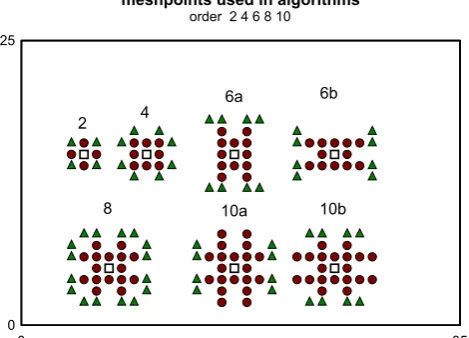
As the average of n algorithms is also an algorithm a minimal algorithm may be formed from a set of base points together with one additional point. In figure 2 the set of points used in forming this algorithm is displayed for various algorithm orders.

Fig. 2. The set of required mesh points for an algorithm of the indicated order. Both order 6 and order 10 need two base sets as discussed in the text.

z axis

r axis

cylinder with boundaries lying on meshpoints

-2 -1 0 1 2 3 4 5 6 7 8 9 10 11 12 0

2 4 6 8 10 12

0v 0v

10v

meshpoints used in algorithms

order 2 4 6 8 10

0 35

0 25

2 4

6a 6b

For example, in the order 4 algorithm there are 9 required points, 8 of these are base points given by the solid discs and 1 is taken from any of the trianglular points. Since each 9 point set is a separate algorithm, the average algorithm is the sum of the 8 single algorithms each of these algorithms taking a separate additional triangular point.

Seen in figure 2 when forming the order 6 and 10 algorithms two separate base sets are used. Further it is readily seen that the actual meshpoints in the minimal algorithm for orders 6, 8, and 10 are identical to those of the order 8 algorithm.

IV. THE MESHPOINT COVERING

For the majority of mesh points shown in figure 1, the required neighboring meshpoints exist for any of the algorithms of figure 2. However for meshpoints one unit from any boundary (see point r=5, z=9 of figure 1) any algorithm of order >2 would not have the necessary neighboring meshpoints. This limitation has been one of the fundamental difficulties of the FDM technique. The strategy used here is to place by construction meshpoints on the other side of the boundary and hence overcoming this restriction.

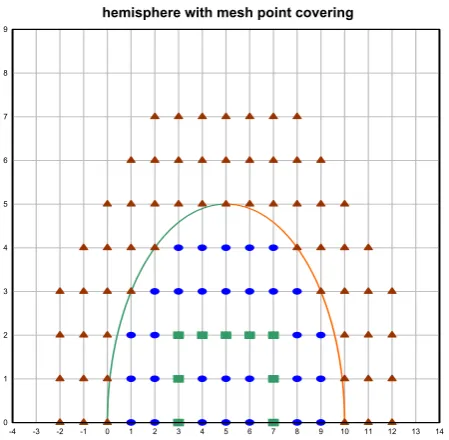
When constructing the meshpoint overlay of the geometry, the covering is extended sufficiently beyond the geometric boundary so that any meshpoint internal to but near the boundary would have the required meshpoints for any order algorithm. An example of such a covering for the discontinuous hemisphere is shown in figure 3.

Fig. 3. A concentric sphere is shown consisting of two hemispheres at different potentials thus creating a singular point at their junction.

A. Determining values of the external points

The value of any external point s is found as follows: first

find the closest boundary point b to the point s. Then select

point c, an ingeometry point closest to point b, while also

being j units from the boundary (see figure 3). The electric field surrounding point c is then determined and extended to

the region between s and b and thus the value at s can be

found by integrating this field from b to s. The separation of

point c from b is necessary for stability considerations as

discussed in [8]. A useful separation of point c from the

boundary has been found to lie between 2 and 3 units. The details of calculation can be understood by referring to

figure 4 in which a curved boundary is shown together with an external point s, a boundary point b closest to s, and the

point c about which the field is calculated. It is noted that

the coordinates of all points in figure 4 are in absolute mesh units.

Fig. 4. In this figure are depicted three points: an external point to the boundary at s, the closest boundary point b to s, and an ingeometry point about which the electric field is to be determined.

Simplifying the notation of (1), the potential at any point x

in an nhbd ofc may be written as:

, ∑ , (4)

being the index of the last term in (1), r and z being the relative coordinates wrt point c. Further is the value

at the mesh point c, , is rl_*zm _{for the kth term in the}

expansion (1), and the index of the last term in (1). Note that will depend upon the order of the algorithm used.

Now the potentials at b and s may be explicitly written in

terms of the coefficients ck:

∑ rb , zb (5)

∑ rs , zs (6)

Letting r , z be the coordinates of point c. The coordinates of b or s relative to point c may be written:

r , z (7)

for x being either b or s.

Using (3), (5), and (6) it is found after a brief calculation:

∑∈ _ ∗ (8)

Where:

_ ∑ coeff_b , k ∗ , , , (9)

Defining by:

, , , , , (10)

Thus at the end of the day an equation for vs is formulated in terms of a summation over the neighboring meshpoints, each meshpoint multiplied by coeff_bj. This is of identical form as the expression for the evaluation of all of the ingeometry meshpoints (see (3)) and is useful in the software development as the coefficients may be calculated only once during mesh initialization for each external point and not during the runtime iteration process. It may be

mesh pt covering external internal and ingeom far.grf hemisphere with mesh point covering

-4 -3 -2 -1 0 1 2 3 4 5 6 7 8 9 10 11 12 13 14

0 1 2 3 4 5 6 7 8 9

curve plus 3 points grf

0 20

0 20

s (rs,zs)

b (rb,zb)

worthwhile to remark that when determining the value of s,

the neighboring mesh points used in the algorithm are those surrounding c and not the neighbors of s itself since the

coefficients ck used in (8) in determining the value of mesh

point s depended uponthe neighbors of point c.

In summary the values of ingeometry points are found using equation 3 while those for external points equation 8 is used. It is noted that for any order only one algorithm is necessary, namely the average or minimal algorithm regardless of the situation in which it is applied.

V. NEUTRALIZING THE EFFECT OF THE SINGULARITY

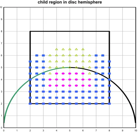
It was found as mentioned in the introduction that by increasing the point density surrounding a singularity, the errors resulting from the singularity would be mitigated. To this end one needs create a structure of regions telescoping into the singularity each region in the structure having an enhanced density (x4) over the density of its parent. The first step in this process is to create a child region about the singularity which is defined by a bounding rectangle centered on the singularity. The points within the child are placed at integer and half integer points within this rectangle. This is illustrated in figure 5 in which a single child region is placed about the juncture of the two hemispheres – a singular point - at r=5, z=5. For illustration the height and width is taken to be 6 units. Shown in this figure are: the internal, external, and shadow points of the child region.

Figure 5. A child region is shown defined by a bounding rectangle and centered on the singular point. Also present are the shadow points (squares), external points (triangles), and ingeometry points (discs).

As the child itself is considered to be a Dirichlet region the values on its enclosing boundary must be evaluated before the region is relaxed. The boundary points of the region are constructed by not only taking those points lying on the bounding rectangle but in addition the 2 internal rows, the complete set of boundary points being named shadow points. This construction is effected so that when relaxing any ingeometry point of the child the c0 algorithm

may be used (equation 3) as the complete 3 rings of neighboring meshpoints are by construction available. To determine the value of any external non shadow point of the

child region the analysis given in IV applies and equation 8 is used. And likewise for any internal non shadow point equation 3 is used.

Special consideration must be given the shadow points themselves. If the shadow point is an even point (its

coordinates being even) then it is the image of a parent point and hence the parent’s value is assumed. For non-even

ingeometry shadow points, their values are set by integration to it from the closest parent point c on the bounding

rectangle, this point also being greater than ~2 units from the geometric boundary. For non-even external shadow

points their values are also set by integration to it from the closest point on the geometric boundary using the field surrounding a parent point c on the bounding rectangle again

~ 2 units from the geometric boundary.

In this manner all shadow points are set from the parent’s net before the child is relaxed. The child itself is then relaxed in the same manner as the parent discussed in I. Again it is remarked that for any order onlyone algorithm is used regardless of the variety of tasks to be performed.

One proceeds with the creation of the next child by induction, i.e. one treats the child region as the parent of its child and continues as described above. This process is then repeated until a specified number of regions have been established. As an example, a region structure consisting of a chain of 10 regions is shown in figure 6 for Router of 360, Rinner of 180, and an hw of each child of 120 (hw = height=width of the bounding rectangle).

Figure 6. The concentric sphere geometry with a singularity at the juncture of the two outer hemispheres is shown. A measurement sphere of radius 300 is also drawn being used in the section of the testing of precision.

In this work the region structure is created by defining the total number of regions in the chain, the hw parameter for the 1st _{child and the last child. Then the hw for each region}

is required to vary linearly from the first to the last child. This construction takes into account that the errors in the jth

region in the chain, depending on its region index, will be have a reduced effect on the precision of the values in the main net. Thus this strategy for region structure definition represents a reasonable, although likely not optimal, compromise between error reduction and memory allowance. It is shown in the next section that a high precision result is be obtained using this approach.

single region parent points child points shadowpointst.grf

child region in disc hemisphere

0 1 2 3 4 5 6 7 8 9 10

0 1 2 3 4 5 6 7 8 9 10

z axis

r axis

disc sphere with 10 child regions

Rinner = 180 Router = 360 hw = 120 measurement sphere 300

0 60 120 180 240 300 360 420 480 540 600 660 720 780 0

60 120 180 240 300 360 420

v=0

v=0

v=10

VI. TESTING THE PRECISION OF THE MULTI REGION STRUCTURE

The discontinuous concentric sphere is one of the few singular geometries having a known solution (see Jackson [9]) and is used in our tests of precision. The parameters defining this geometry together with the region structure defined above are: Rout = radius of outer sphere, Rin = radius of inner sphere, nt = total number of child regions, hw (j) the width and height of the bounding rectangle of the jth

child. The highest precision which was obtained by taking nt = 36, hw (0) = 120, and hw (nt) = 40. With these parameters, the error spectra on measurement spheres both near the outer and inner boundaries are given in figure 7 for algorithms of order 2 and 10.

Figure 7. The error spectra measured along test spheres both near the outer and inner spheres for both order 2 and order 10 algorithms used in the process. Apparent is the clear separation in precisions between the order 2 and 10 algorithms

Figure 7. The error spectra measured along test spheres both near the outer and inner spheres for both order 2 and order 10 algorithms used in the process. Apparent is the clear separation in precisions between the order 2 and 10 algorithms

Fig 7. The error spectra measured along test spheres both near the outer and inner spheres for both order 2 and order 10 algorithms used in the process. Apparent is the clear separation in precisions between the order 2 and 10 algorithms.

Seen is that the maximum error for the order 10 algorithm is ~10-16 _{and occurs near the outer boundary as expected.}

The maximum error in both plots has been found to decrease monotonically for measurement spheres going from the outer to inner one. The cusps present in these spectra are likely due to the change of the sign of the error as the error point proceeds along the path on the measurement sphere. Since the error spectra is a continuous function the error will be close to 0 somewhere between this sign change in the error spectra.

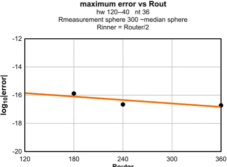
Similar physical geometries may be obtained by multiplying both the inner and outer radii by a scale factor and the result of the maximum error along a measurement sphere approximate to the median sphere of the scaled geometry is shown in figure 8.

Fig 8. The maximum error is plotted vs the value of Rout for the measurement spheres being ~ the median sphere for a constant region structure.

Seen in this figure is that the maximum error is a weak function of the density of the main net.

The maximum error over the geometry Rout=360, Rin=180 was measured as a function of the order of the algorithm used in the relaxation process and is given in fig. 9.

Figure 9. To obtain the data for this figure the geometry was fixed and the maximum error plotted as a function of order for either the main net only (no child regions) or for the 36 region structure (lower curve).

The dependence on the maximum error on order is thus seen to be strong for the process using the 36 region structure. However for relaxing the main net without any child regions essentially no reduction in the error is found as a function of algorithm order. This is a result consistent with the early attempts mentioned in the introduction at improving the relaxation precision with more precise algorithms and emphasizes the necessity of not only using high order algorithms but using them with an appropriate region structure in order to effect high precision results. The other rather remarkable and perhaps surprising feature seen in figure 9 is that the resultant error of the order 2 algorithm is independent on whether or not a 36 region structure is incorporated into the geometry. Said somewhat differently no gain in the precision can be obtained when using a low order algorithm by attempting to neutralize the singularity using telescopic child regions.

To investigate the dependence of the maximum error on hw (0), hw(0) was varied while hw (nt) was taken to be 40

z axis

lo

g10

|

error)

error plot for discontinuous concentric sphere Router = 360 Rinner = 180

hw(0) = 120 hw(nt) = 40 nt = 36 Rmeas 355 and 190

0 60 120 180 240 300 360 420 480 540 600 660 720 -21

-19 -17 -15 -13 -11 -9 -7 -5 -3 -1

order 10 order 2

Router

log

10

|error|

maximum error vs Rout hw 120--40 nt 36

Rmeasurement sphere 300 ~median sphere Rinner = Router/2

120 180 240 300 360

-20 -18 -16 -14 -12

order

log

10

| max error|

max error vs order for ~median measurement sphere nt either 36 or 0 hw 120 -- 40

Rms = 300

0 2 4 6 8 10 12

-18 -16 -14 -12 -10 -8 -6 -4 -2

no child regions

independent of hw(0), for nt of 36. The result is shown in figure 10.

Fig. 10. The maximum error on the indicated measurement sphere is found and plotted vs hw(0).

Seen in this figure that to achieve precisions greater than ~10-12 _{hw (0) must be larger than 40.}

To evaluate the dependence of the precision of an order 2 algorithm on relaxation time the discontinuous concentric sphere was overlaid with meshes of various densities (from Rout = 480 to 120, Rin = Rout/2), the particular mesh relaxed (using an end criterion of 2*10-12_{) and both the}

relaxation time and the maximum error on a median measurement sphere determined and plotted in figure 11. It is noted that no child regions were incorporated since their effect on the precision of the order 2 algorithm has been seen to be negligible (see figure 9).

Figure 11. The main net having been created for various discontinuous concentric sphere geometries was relaxed using an order 2 algorithm and the maximum error on a median measurement sphere plotted vs the time to relax the net. A linear interpolation of the data to large relaxation times has been made.

Seen from this figure that to achieve precisions of the order 10-10 _{would require relaxation times of the order 10}19

seconds and a time in excess of the age of the universe. This example demonstrates the difficulty of achieving high precisions using an order 2 algorithm.

VII. SUMMARY AND CONCLUSION

The process of neutralizing the effect of singularities on a curved boundaries has been described. The solution has necessitated the creation of a telescoping set of regions of ever higher density converging on the singular points themselves.

It has been shown that the effect of these singular points can be neutralized to a level of ~10-16 _{using an order 10}

algorithm together with a telescoping region structure consisting of 36 child regions.

The conclusion is clear, namely, that a very precise potential distribution interior to curved singular boundaries can be found using the finite difference method.

This paper both completes and concludes the effort which the author began in ~1980 to calculate electrostatic potentials for arbitrary geometries to a very high precision. Newark December 24, 2014

REFERENCES

[1] Anjam Khursheed, The finite element method in charged particle

optics, Kluwer Academic Publishers, ISBN 0-7923-8611-6, 1999.

[2] E. Durand C. R. Acad. Sci. Paris, 244, 2355-2358. [3] S. Natali, D. Di Chio, C.E.Kuyatt,

[4] S. Natali, D. Di Chio, C.E.Kuyatt, “Accurate Calculations of Properties of the Two-Tube Electrostatic Lens”, J. Res. Nat. Bur. Stand. Sect. A, 76, 27 (1972).

[5] C. E. Kuyatt, A. Galejs, “Tests of Fourth-Order Difference Equations for Laplace’s Equation in Cylindrical Coordinates”, Science Technol. 78, 655 (1978).

[6] David Edwards, Jr. “Accurate calculations of electrostatic potentials for cylindrically symmetric lenses”, Rev. Sci. Instr., 54, 1, 729 (1983).

[7] David Edwards, Jr., “High precision electrostatic potential calculations for cylindrically symmetric lenses”, Rev. Sci. Instr., 78, 1-10 (2007)

[8] David Edwards, Jr., Proceedings of the International Multi Conference of Engineers and Computer Scientists 2014, Vol I, IMECS 2014, March 12 - 14, 2014, Hong Kong

[9] D.W.O.Heddle, Electrostatic Lens Systems, 2nd ed., 2000, Institute of

Physics Publishing, ISBN 0-7503-0697-1, pp 32 to60.W.-K. Chen, Linear Networks and Systems (Book style). Belmont, CA: Wadsworth, 1993, pp. 123–135.

[10] John David Jackson, Classical Electrodynamics, John Wiley & Sons, New York, London, 1963 (Library of Congress card number 62-8744).

hw(0)

log

10

|error|

maximum error vs hw(0)

nt = 36 hw(nt) = 40 Rmeasurement sphere = 300

0 20 40 60 80 100 120 140

-20 -18 -16 -14 -12 -10 -8 -6 -4 -2

log relax time(seconds)

log | error |

error vs relax time order 2 main net

0 2 4 6 8 10 12 14 16 18 20 22 24 26 28 30 -3

-4 -5 -6 -7 -8 -9 -10 -11 -12 -13 -14 -15