Empirical Optimal Kernel for Convex Multiple
Kernel Learning
Peiyan Wang, Dongfeng Cai, Guiping Zhang, Yu Bai, Fang Cai, Tianhao Zhang
Abstract—Multiple kernel learning (MKL) aims at learning a combination of different kernels, instead of using a single fixed kernel, in order to better match the underlying problem. In this paper, we propose the Empirical Optimal Kernel for convex combination MKL. The Empirical Optimal Kernel is based on the theory of kernel polarization, and is the one with the best generalization ability which can be achieved from the training data in the convex combination scenario. Based on the Empirical Optimal Kernel, we propose three different algorithms: heuristic approach, optimization approach and alternating optimization approach to find the optimal com-bination weights. On Multiple Features Digit Recognition data set, the proposed methods achieve comparative performance as the compared methods, and have less support vectors and active kernels. On 5 UCI data sets, the Empirical Optimal Kernel based optimization approach has higher winning percentage (t-test with significant level 0.05), less active kernels and support vectors than the other MKL algorithms.
Index Terms—multiple-kernel-learning, convex-combination, empirical-optimal-kernel.
I. INTRODUCTION
K
ERNEL methods have delivered high performance in a variety of machine learning tasks [1]. The key to success is the incorporation of the kernel trick which amounts to an implicit mapping of data into a feature space (usually higher dimension). The implicit mapping is determined by specifying a kernel function, which calculates the inner product between each pair of data points in the feature space.k(xi,xj) =hφ(xi), φ(xj)i φ:X→H (1) where X is the original data space and H is the feature space. The main advantage of kernel methods is the ability to use linear algorithms in feature space and the nonlinearity is implicitly introduced by the kernel function. Despite the success of kernel methods, choosing the appropriate kernel function is crucial. In recent years, multiple kernel learning (MKL) methods have been proposed, aiming at learning an optimal combination of a set of predefined base kernels in order to identify a good target kernel for the applications [2]. Compared with traditional kernel methods using a single fixed kernel, MKL does exhibit its flexibility of automated kernel learning, and also reflects the fact that typical learning problems often involve multiple, heterogeneous data sources.
Manuscript received July 10, 2014; revised July 29, 2014. This work was supported in part by National Key Technology R&D Program of China (2012BAH14F00).
Peiyan Wang is with the College of Computer Science and Technology, Nanjing University of Aeronautics and Astronautics, Nanjing, 210016, China, e-mail: (wangpy [email protected]).
Peiyan Wang, Dongfeng Cai, Guiping Zhang and Yu Bai are with the Knowledge Engineering Research Center, Shenyang Aerospace University, Shenyang 110136, China.
Fang Cai and Tianhao Zhang are with the EECS, University of California, Berkeley.
In other words, since the base kernels can be built from different types of data representations, the MKL approach has the advantages of the possibility to combine and select the most relevant data representation in an elegant way.
Generally, the vast majority of analyses and algorithms for MKL focus on learning finite linear combinations of given base kernels:
kη(xi,xj) = p X
m=1
ηmkm(xi,xj) (2)
where η denotes the kernel weights. Different versions of this approach differ in the way ones put restrictions on the kernel weights. For example, one can use arbitrary weights (η ∈ Rp, linear combination) [3], non negative kernel weights (η ∈ Rp+, conic combination) [4][5], or weights on a simplex (η∈Rp+ andPp
m=1ηm= 1, convex combination) [6]. The convex has advantage over the linear sum in terms of interpretability. We can extract the relative importance of the combined kernels by looking at their weights. Convex combination is widely used in many fields, such as information extraction [7] and bioinformatics [8].
In this paper, we only focus on the convex multiple kernel learning. Based on the theory of kernel polarization [9], we propose the Empirical Optimal Kernel for convex combination MKL. The Empirical Optimal Kernel is the one with the best generalization ability which can be achieved from the training data in the convex combination scenario. In order to apply the Empirical Optimal Kernel in MKL, we propose three different algorithms: heuristic approach, optimization approach and alternating optimization approach. The experimental results demonstrate the effectiveness of the Empirical Optimal Kernel.
The rest of this paper is organized as follows: Section 2 describes the kernel polarization and the Empirical Optimal Kernel in detail. Section 3 proposes the MKL algorithms to utilize the Empirical Optimal Kernel. Experimental results are presented in Section 4, and the last section gives some concluding remarks.
II. THE PROPOSED METHOD
In this section, we firstly describe the kernel polarization in detail, including the advantage and the limitation. Sec-ondly, we propose the Empirical Optimal Kernel for convex combination MKL based on kernel polarization.
A. Kernel Polarization
xi ∈ X ⊂Rn (The input space) and yi ∈ {−1,+1}. The definition of kernel polarization is:
P(K) = 1 l2
l X
i=1
l X
j=1
yiyjk(xi,xj) (3)
Clearly, P(K) will increase if points in the training set with the same label come closer and points with different labels are more separated, in the sense that the kernel is a proximity measure [9]. Kernel polarization possesses several convenient theoretical properties. First, it is efficient in that its computational complexity is O(n2)in terms of the size of training set. With a simple formula, it can be an objective function of an optimization problem [10]. Furthermore, there exists a separation of the data with a low bound on the generalization error, if the polarization is complete, in the sense that P(K) attains its absolute maximum value. One limitation of the kernel polarization is that the kernel should be a proximity measure [9]. This will be the case if, for instance, the kernel is a continuous monotone function of the Euclidean distance between its two arguments. Furthermore, the maximization problem will be well posed if the feature space is confined. Most common kernel functions possess the properties above, such as Gaussian kernel, Exponential kernel [11] and Bessel Kernel [12].
B. Empirical Optimal Kernel
According to the theory of the polarization, the best kernel for a particular application is the one with the maximum kernel polarization value. Given training samples, based on (Eq. 3), the maximum kernel polarization is:
max{P(K)}=max{1
l2
l X
i=1
l X
j=1
yiyjk(xi,xj)}
=max1 l2{
X
yi=yj
k(xi,xj)− X
yi6=yj
k(xi,xj)}
∝max{X
yi=yj
k(xi,xj)− X
yi6=yj
k(xi,xj)}
=max{X
yi=yj
k(xi,xj)}+max{− X
yi6=yj
k(xi,xj)}
=max{X
yi=yj
k(xi,xj)} −min{ X
yi6=yj
k(xi,xj)}
= X
yi=yj
max{k(xi,xj)} − X
yi6=yj
min{k(xi,xj)} (4)
Equation (4) shows that the best kernel is the one that gives its maximum value to point pairs from same classes, and gives its minimum value to point pairs from different classes. The kernel matrix of the best kernel is:
[K]i,j =
max{k(xi,xj)} yi=yj
min{k(xi,xj)} yi6=yj
(5)
Taken Gaussian kernel for instance, in theory, the maximum value is ”1” and minimum value is nearly ”0”. The kernel matrix of the best Gaussian kernel is:
[K]i,j=
1 yi=yj
0 yi6=yj (6)
It is the same as the ideal kernel proposed in [13]. In practice, it is hard to achieve the best condition for single kernel, since the maximum or minimum kernel value for two data points could not be determined exactly. However, in the convex combination MKL scenario, the maximum or minimum value of combined kernel is fixed, due to the determination of the base kernel.
For convex combination MKL (Eq. 2),kη can be seen as the weighted average of base kernelskm. Given the finite set of base kernels, for any two data points:
kmin(xi,xj)≤kη(xi,xj)≤kmax(xi,xj) (7) where kmin and kmax denote the minimum value and the maximum value of{k1(xi,xj), k2(xi,xj), ...km(xi,xj)} re-spectively.
Summarizing the above, we give the optimal kernel for convex combination MKL:
kopti(xi,xj) =
kmax(xi,xj) yi=yj
kmin(xi,xj) yi6=yj
(8)
We name it ”Empirical Optimal Kernel”, because the defini-tion of the optimal kernel is based on the base kernels and the training data.
C. Generalization Ability of Empirical Optimal Kernel
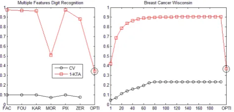
In this section, we evaluate the generalization ability of Empirical Optimal Kernel by Kernel Target Alignment (KTA, Eq. 9) [14]. There exists a separation of the data with a low bound on the generalization error, provided that the expected value of KTA is high. Fig. 1 illustrates the 10 cross-validation error rate and 1-KTA value using Gaussian kernel (σ = 1) for different features on Multiple Features Digit Recognition data set. It also illustrates the 10 cross-validation error rate and 1-KTA value using 21 different Gaussian kernels (σ= 1,20,30, ...,200) for the same feature representation on Breast Cancer Wisconsin data set.
A(K, yyT) = hK, yy
Ti F p
hK,KiF· p
hyyT, yyTi F
(9)
From Fig. 1, we can see that 1-KTA varies similarly to CV error rate, and the two curve have the same tendency. KTA is correlative well with error rate and can reflect the generalization ability. It also can be seen that the Empirical Optimal Kernel (opti) has the lowest 1-KTA value, is much lower than the best case of each data set ( ”FAC” for Multiple Features Digit Recognition, σ = 1 for Breast Cancer Wisconsin ). In conclusion, the Empirical Optimal Kernel would have good generalization ability and better than each base kernel.
III. MKLALGORITHMS BASED ONEMPIRICALOPTIMAL KERNEL
Fig. 1. 1-KTA and CV error rates on Multiple Features Digit Recognition and Breast Cancer Wisconsin data set
For MKL, a recent approach is to use a two-stage pro-cedure [5],[15], in which the first stage finds the optimal weights to combine the kernels, and the second stage trains a standard classifier using the combined kernel. In a more general point of view, such MKL should be considered as a model selection problem: the kernel weights are the hyperparameters of the classifier and are tuned based on the model selection criteria [16],[17]. One significant property of the two-stage approach is that, in the first stage, it makes use of the information from the entire training data and can be computed efficiently. In the two-stage strategy, we apply the Empirical Optimal Kernel to find the optimal weights in the first stage. To achieve this, we propose three different algorithms: heuristic approach, optimization approach and alternating optimization approach.
A. Heuristic Approach
The Empirical Optimal Kernel is based on the base ker-nels. Thus, we give higher weight to the base kernel which is more contributed to the Empirical Optimal Kernel. We apply kernel alignment to measure how well a base kernel matches with the Empirical Optimal Kernel:
ηm=
A(Km,Kopti) p
P
h=1
A(Kh,Kopti)
(10)
A(Km,Kopti) =
hKm,KoptiiF p
hKm,KmiFphKopti,KoptiiF (11)
where Km and Kopti denote the kernel matrix for base kernel and the empirical optimal kernel respectively. This approach is similar with the method proposed in [18].
B. Optimization Approach
Optimization approach is similar with [19] and solves a QP problem in (Eq. 12)
min
p P
m=1
p P
h=1
ηmηhhKm,KhiF−2 p P
m=1
ηmhKm,KoptiiF
w.r.t.η∈p+
s.t.
p P
m=1 ηm= 1
(12) Optimization approach (Eq. 12) not only considers the align-ment between one base kernel and the Empirical Optimal Kernel but also the similarity with other base kernels. It will
give higher weight to kernels that contribute more to the Empirical Optimal Kernel and diverge more from other base kernels.
C. Alternating Optimization Approach
The Empirical Optimal Kernel is associated with each point pair in the training data, so that it can involve the local properties of the data, but it is also sensitive to the noisy data. We set a coefficient to each point of training data to reflect the importance of the point. The kernel with coefficient is:
k0(x1,x2) =hα1·φ(x1), α2·φ(x2)i =α1α2hφ(x1), φ(x2)i
=α1α2·k(x1,x2)
(13)
The kernel matrix is:
K0= A◦K
[A]ij =αiαj SubstituteK0 forK in (Eq. 12):
min
p P
m=1
p P
h=1
ηmηhhK0m,K0hiF−2 p P
m=1
ηmhK0m,K0optiiF
w.r.t.η∈p+
s.t.
p P
m=1 ηm= 1
(14) We obtainαfor each data point by solving the QP problem of SVM:
maximum
l P
i=1 αi−12
l P
i=1
l P
j=1
αiαjyiyjkη(xi,xj)
w.r.t.α∈[0, C]l
s.t.
l P
i=1
αiyi= 0
(15)
It is an alternating optimization procedure, which determines ηby solving (Eq. 14) initially, then substitute it in (Eq. 15) and getα, solve (Eq. 14) again to obtain newη, repeat this process untilη is stable.
This approach assumes that the support vectors are the most important points, and setα= 0for the other points. It can effectively filter the noisy data. However, it still cannot effectively involve the local properties of the Empirical Op-timal Kernel. It needs further research on utilizing the local property of the Empirical Optimal Kernel and on ignoring the noise.
IV. EXPERIMENTS
In this section, we report experimental performance of OBMKL (empirical Optimal kernel Based MKL) for classi-fication on Multiple Features Digit Recognition data set and 5 UCI data sets. All data is scaled to[−1,+1]. Classification is performed using the SVM from the LIBSVM1 library and the regularization parameter C is chosen from the set
{0.1,1,10,100,1000}by 5-fold cross validation on training data. We use 10-fold cross validation to estimate the error rates.
A. Compared Algorithms
We compare proposed method with RBMKL, ABMK-L(ratio), ABMKL(convex), GMKL and GLMKL. These Al-gorithms are all for convex multiple kernel learning. We use the MATLAB implementations of RBMKL, ABMKL, GMKL and GLMKL proposed in [2] and the SVM classifiers are trained using LIBSVM.
RBMKL denotes rule-based MKL algorithms, trains an SVM with the mean of the combined kernels.
ABMKL(ratio) denotes alignment-based MKL algorithms. To determine the kernel weights, ABMKL(ratio) uses the heuristic in (Eq. 16) [18], ABMKL(convex) solves the QP problem in (Eq. 17) [19]. In the second step, all methods train an SVM with the kernel calculated with these weights.
ηm=
A(Km, yyT) P
P
h=1
A(Kh, yyT)
(16)
min
P P
m=1
P P
h=1
ηmηhhKm,KhiF −2 p P
m=1
ηmKm, yyTF
w.r.t.η∈p+
s.t.
p P
m=1 ηm= 1
(17) GMKL is the generalized MKL algorithm in (Eq. 18) [20]. In the implementation, ris the convex combination of base kernels and is taken as 1/2(η−1/p)T(η−1/p).
maxJ(η) =
N P
i=1 αi−12
N P
i=1
N P
j=1
αiαjyiyjkη(xi,xj) +r(η)
w.r.t.α∈N
+
s.t.
N P
i=1
αiyi= 0, C ≥αi≥0∀i
(18) GLMKL denotes the group Lasso-based MKL algorithms proposed by [21] and [22]. While set the parameterp= 1, GLMKL updates the kernel weights using (Eq. 19) and learns a convex combination of the kernels.
η= kwmk2
P P
h=1
kwhk2
,kwmk22=η2 N X
i=1
N X
j=1
αiαjyiyjkm(xmi , x m j )
(19)
B. Multiple Features Digit Recognition Experiments
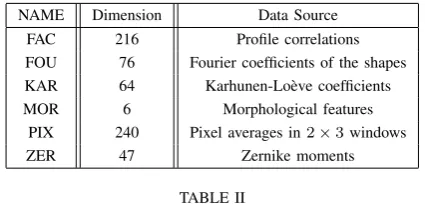
[image:4.595.320.533.78.180.2]We conduct experiments on the Multiple Features (MUL-TIFEAT) Digit Recognition data set from the UCI Machine Learning Repository, composed of six different feature repre-sentations for 2,000 handwritten numerals. The properties of these feature representations are summarized in Table 1. We use Gaussian kernels with parameter σ = 1 for all feature sets. The purpose of choosing this data set is to exam the ability of the proposed method in identifying the appropriate combination of different feature subsets.
Table 2 gives the results of all algorithms on the MUL-TIFEAT data set. OBMKL(ratio) denotes heuristic approach based on Empirical Optimal Kernel, OBMKL(qp) denotes
TABLE I
MULTIPLE FEATURE REPRESENTATIONS IN THEMULTIFEATDATA SET.
NAME Dimension Data Source FAC 216 Profile correlations FOU 76 Fourier coefficients of the shapes KAR 64 Karhunen-Lo`eve coefficients MOR 6 Morphological features
PIX 240 Pixel averages in2×3windows
ZER 47 Zernike moments
TABLE II
PERFORMANCES OFMKLALGORITHMS ON THEMULTIFEATDATA
SET USING THEGAUSSIAN KERNEL.
CV SV AK
OBMKL (ratio) 0.0679±0.0364 392.1±161.2 6±0
OBMKL(qp) 0.0677±0.0380 301.8±174.8 2±0
OBMKL(aqp) 0.0584±0.0324 418.6±179.8 2±0
ABMKL(ratio) 0.0681±0.0367 375.9±164 6±0
ABMKL(convex) 0.0716±0.0403 243.1±136 1.2±0.4
GMKL 0.0573±0.0282 647.8±410.5 3.4±1.2
GLMKL 0.0582±0.0285 668.5±422 5.8±0.4
RBMKL 0.0661±0.0330 760.2±161.2 6±0
SVM(best) 0.0628±0.0325 889.9±711.9 1±0
optimization approach, and OBMKL(aqp) denotes alternat-ing optimization approach. SVMs are trained on each feature representation singly, and the one with the lowest average validation error is referred as SVM(best). The number of active kernels (AK) and the number of support vectors (SV) are also listed in Table 2. GMKL has the lowest average error rate than others, but is not significantly lower than OBMKL(aqp) and GLMKL (t-test with significant level 0.05). However, the active kernels number and support vec-tors number of OBMKL(aqp) are much smaller than GMKL and GLMKL. It implies that OBMKL(aqp) would spend less time on the prediction stage, and would have better generalization ability. ABMKL(convex) has the least active kernels number alone with the least support vectors number, but receives the highest average error rate. It may be due to over-fitting. In addition, GMKL, GLMKL and OBMKL(aqp) outperform SVM(best). This shows that MKL is helpful in identifying the appropriate combination of data sources or different feature subsets in real-world applications. Above all, the Empirical Optimal Kernel and the corresponding algorithms based on it are effective for multiple features combination classification. With less active kernel number and support vector number, the proposed methods achieve comparative performance as the compared methods.
C. UCI Data Sets
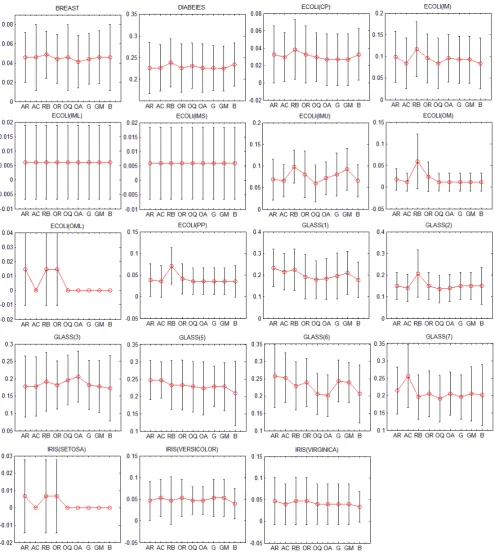
Fig. 2. Performances of MKL algorithms on the UCI data set using the 21 Gaussian kernels. (AR, AC, RB, OR, OQ, OA, G, GM and B denote ABMKL(ratio), ABMKL(convex), RBMKL, OBMKL(ratio), OBMKL(qp), OBMKL(aqp), GMKL, GLMKL and SVM(best) respectively)
one with the lowest average validation error as SVM(best). Fig. 2 lists 10-fold cross validation error rates.
Two-tailed t-test with the significant level 0.05 is per-formed to determine whether there is a significant difference between the proposed method and other methods. A win-tie-loss (W,T,L) summarization based on t-test is listed in Table 3. A win or a loss means that one method is better or worse than another method on a data set. A tie means that both methods have the same performance. For example, ”6,8,5” in ”OBMKL(ratio)” column and ”ABMKL(ratio)” row means
OBMKL(ratio) is better than ABMKL (ratio) in 6 out of 19 binary classifications, is worse in 5 binary classifications, and has same performance in 8 binary classifications.
TABLE III
PERFORMANCES OFMKLALGORITHMS ON THEUCIDATA SET USING
THEGAUSSIAN KERNEL.
OBMKL(ratio) OBMKL(qp) OBMKL(aqp)
OBMKL(ratio) - 14,2,3 13,4,2
OBMKL(qp) 3,2,14 - 5,8,6
OBMKL(aqp) 2,4,13 6,8,5
-ABMKL(ratio) 6,8,5 13,4,2 13,4,2 ABMKL(convex) 5,4,10 7,9,3 7,8,4
GMKL 2,8,9 8,7,4 7,9,3
GLMKL 3,6,10 7,9,3 7,8,4
RBMKL 10,5,4 15,3,1 14,3,2
SVM(best) 3,3,13 6,7,6 5,5,9
Total 34,40,78 76,49,27 71,49,32
Win% 22.37% 50% 46.71%
TABLE IV
WINNING PERCENTAGES OFMKLALGORITHMS.
Total Win% SV AK
OBMKL(ratio) 34,40,78 22.37% 189.1±107.7 21±0
OBMKL(qp) 76,49,27 50% 106.9±99.5 2.3±0.4
OBMKL(aqp) 71,49,32 46.71% 140.6±101.2 2.8±0.5
ABMKL(ratio) 28,40,84 18.42% 182.1±113.7 21±0
ABMKL(convex) 53,54,45 34.87% 113.5±107.2 1.7±0.7
GMKL 57,54,41 37.5% 166.7±125.2 19.3±3.4
GLMKL 56,56,40 36.84% 173.4±128.5 21±0
RBMKL 22,25,105 14.47% 252.1±122.3 21±0
SVM(best) 83,41,28 54.61% 181.3±114.5 1±0
summarizes the winning percentage of all MKL algorithms. SVM(best) has the highest winning percentage, OBMKL(qp) and OBMKL(aqp) are higher than the others. Table 4 also lists the average active kernels number (AK) and the average support vectors number(SV). It is shown that OBMKL(qp) has the least support vectors, its active kernels number is significantly lower than the others expected ABMKL(convex) and SVM(best). OBMKL(qp) has higher winning percentage, less active kernels number and support vectors number than the other MKL algorithms.
V. CONCLUSION
In this paper, we propose the Empirical Optimal Kernel for convex combination MKL. It is the kernel with the best generalization ability which can be achieved from existing training data in the convex combination scenario. Then, we propose three different algorithms: heuristic approach, optimization approach and alternating optimization approach, which utilize the Empirical Optimal Kernel in MKL. In ex-periment, we applied the Multiple Features Digit Recognition data set and five UCI data sets to demonstrate the effective-ness of the Empirical Optimal Kernel and the corresponding algorithms. On Multiple Features Digit Recognition data set, the proposed methods achieve comparative performance as the compared methods, and have less support vectors and active kernels. On UCI data sets, the Empirical Optimal Kernel based optimization approach has higher winning percentage, less active kernels and support vectors than the other MKL algorithms.
The Empirical Optimal Kernel is built on each point pair in the training set. Then, it can involve the local property of the
data set, but it is also sensitive to the noisy data. The methods proposed in this paper still cannot effectively involve the local property of the Empirical Optimal Kernel. It needs further research on developing localized algorithm [23] to handle this property. In the future, we will also investigate the extent to which the proposed method would provide us the trade-off between the accuracy and computational efficiency.
REFERENCES
[1] B. Sch¨olkopf and A. Smola,Learning with Kernels. MIT Press, 2002. [2] M. G¨onen and E. Alpaydin, “Multiple kernel learning algorithms,”
Journal of Machine Learning Research, vol. 12, pp. 2211–2268, 2011. [3] C. Igel, T. Glasmachers, B. Mersch, N. Pfeifer, and P. Meinicke, “Gradient based optimization of kernel-target alignment for sequence kernels applied to bacterial gene start detection,”IEEE/ACM Transac-tions on Computational Biology and Bioinformatics, vol. 4, no. 2, pp. 216C–226, 2007.
[4] F. R. Bach, G. R. G. Lanckriet, and M. I. Jordan, “Multiple kernel learning, conic duality, and the smo algorithm,” inThe Proceedings of the 21st International Conference on Machine Learning, 2004. [5] C. Cortes, M. Mohri, and R. Afshin, “Two-stage learning kernel
algorithms,” inThe Proceedings of The 27th International Conference on Machine Learning, 2010.
[6] T. Wang, D. Zhao, and Y. Feng, “Two-stage multiple kernel learn-ing with multiclass kernel polarization,” Knowledge-Based Systems, vol. 48, pp. 10–16, 2013.
[7] S. Sarawagi, “Information extraction,” Foundations and trends in databases, vol. 1, no. 3, pp. 261–377, 2008.
[8] B. Sch¨olkopf, T. Koji, and V. J. Philippe,Kernel Methods in Compu-tational Biology. MIT Press, 2004.
[9] Y. Baram, “Learning by kernel polarization,” Neural Computation, vol. 17, pp. 1264–1275, 2005.
[10] T. Wang, S. Tian, H. huang, and D. Deng, “Learning by local kernel polarization,”Neurocomputing, vol. 72, pp. 3077–3084, 2009. [11] C. Bergeron, T. Hepburn, and C. M. Sundling, “Prediction of peptide
bonding affinity: kernel methods for nonlinear modeling,” in The Proceedings of Computing Research Repository 2011, 2011. [12] R. Chen, “Numerical approximations to integrals with a highly
oscil-latory bessel kernel,”Applied Numerical Mathematics, vol. 62, no. 5, pp. 636–648, 2012.
[13] J. T. Kwok and I. W. Tsang, “Learning with idealized kernels,” in
The Proceedings of The 20th International Conference on Machine Learning, 2003.
[14] N. Cristianini, J. Shawe-Taylor, A. Elisseeff, and J. Kandola, “On kernel-target alignment,”Advances in Neural Information Processing Systems, vol. 14, pp. 367–373, 2001.
[15] C. Cortes, M. Mohri, and A. Rostamizadeh, “Algorithms for learning kernels based on centered alignment,”Journal of Machine Learning Research, vol. 13, pp. 795C–828, 2012.
[16] O. Chapelle and A. Rakotomamonjy, “Second order optimization of kernel parameters,” in The Proceedings of NIPS 2008 Workshop on Kernel Learning: Automatic Selection of Optimal Kernels, 2008. [17] Y. Liu, S. Liao, and Y. Hou, “Learning kernels with upper bounds of
leave-one-out error,” inThe Proceedings of the 20th ACM Conference on Information and Knowledge Management, 2011.
[18] S. Qiu and T. Lane, “A framework for multiple kernel support vector regression and its applications to sirna efficacy prediction,”IEEE/ACM Transactions on Computational Biology and Bioinformatics, vol. 6, no. 2, pp. 190–199, 2009.
[19] J. He, S.-F. Chang, and L. Xie, “Fast kernel learning for spatial pyramid matching,” in Proceedings of the IEEE Computer Society Conference on Computer Vision and Pattern Recognition, 2008. [20] M. Varma and B. R. Babu, “More generality in efficient multiple kernel
learning,” inThe Proceedings of The 26th International Conference on Machine Learning, 2009.
[21] M. Kloft, U. Brefeld, S. Sonnenburg, and A. Zien, “Non-sparse regu-larization and efficient training with multiple kernels,” 2010, technical report, Electrical Engineering and Computer Sciences, University of California at Berkeley.
[22] Z. Xu, R. Jin, H. Yang, I. King, and M. R. Lyu, “Simple and efficient multiple kernel learning by group lasso,” inThe Proceedings of the 27th International Conference on Machine Learning, 2010. [23] M. G¨onen and E. Alpaydin, “Localized algorithms for multiple kernel