I. INTRODUCTION URNING is a type of material processing operation where

Abstract_{— In this paper it is examined the use of finite} elements in predicting the cutting forces of machined parts of stainless steel AISI 316L through turning. The process were held in high speed machining which continuously improves and it has be found application in more and more manufacturing processes like aerospace industry, in die and mold companies and in the last years also in bioengineering in manufacturing hip joint implants. The cutting forces, which were measured through experimental process, were compared with predicted ones from the finite element modulation, and it was exported that they can be predicted with good precision when machining with the FEM model.

Index Terms— FEM analysis, High speed Machining, Cutting Forces, AISI 316L

I. INTRODUCTION

URNING is a type of material processing operation where a cutting tool is used to remove an unwanted material to produce a desired product, and is generally performed on a lathe. In recent decades, considerable improvements were achieved in turning, enhancing machining of difficult-to-cut materials and producing better surface finish. Various methods, such as high-speed machining (HSM), have been in use for considerable time [1]. This is not really a new technology. First investigations have been performed by Salomon in the twenties. However, these investigations were only ballistic analysis. The improvement of machine tools and controls made HSM possible in machining operations in the seventies [2]. However, this method and all metal machining processes are characterised mainly by quick changes in quantified elements. Individual changes do not occur in isolation and they influence each other. The analysis of these changes requires study of the complicated complete systems in their real situations. The study of cutting processes such as turning and facing, from dynamic aspects, is very important. The trend towards the measurement of cutting forces in machining leads to many theoretical and practical problems. Theoretical problems associate mainly with the choice of a suitable technique to measure, and the statistical methods to analyse the components of cutting force to be determined in realtime. Practical problems involve the errors and uncertainties relating to the measurement system used [3].

N. I. Galanis is with the National Technical University of Athens, Athens, Greece (corresponding author to provide phone: +302102510174; fax: +302102580365; e-mail: [email protected]).

D. E. Manolakos is with the National Technical University of Athens, Athens, Greece (e-mail: [email protected]).

The cutting operation is controlled by the parameters vc (cutting speed), d (cutting depth) and f (feed rate). The results obtained include specific quality of a machining surface but also cutting forces and tool wear. Only the knowledge of such results could help us to choose an appropriate set of work piece-cutting force-machine tool for a projected industrial production[4]. In this paper, it will be presented the effect of the aforementioned parameters on the cutting forces, during the HSM manufacturing of metallic femoral head, from stainless steel AISI 316L. The forces were measured by a series of experimental measurements. Furthermore there were analysed by the Finite Element Method using AdvantEdge™ and compared with the experimental results.

The results were analysed through the Analysis Of Variance (ANOVA) in order to eliminate the fault factor and they were also evaluated according to the produced surface roughness.

II. CUTTING FORCES

Material removal described so far is known as orthogonal, producing only two cutting forces; when turning these is axial and tangential. Tangential cutting force is by far the greater and axial cutting force is the force required to keep the cutting edge in contact with the. Oblique cutting introduces a third cutting force, radial. It is known that the cutting edge is not perpendicular to the axis of rotation as in orthogonal turning. Tangential cutting force resists the rotation of the work, as relatively high speeds are used the bulk of power consumption lies here. Axial cutting force resists the travel of the tool, however this is a relatively low speed compared with rotation of the work, so for all practical purposes power consumption may be ignored [5].

Furthermore investigations have shown that increasing cutting speed leads to reduced cutting forces and better surfaces. The effect of the cutting speed increase on the cutting forces during the turning process is the reduction of forces. Tests proved that for every investigated steel the cutting force decreases down at approximately 450N when the cutting speed increases up to 500 m/min with feed rate 0.1 mm/rev and cutting depth at 1mm. For the steel with the larger grain sizes, higher forces are to be applied in each case of material separation. At cutting speeds above approximately 800 m/min no further reduction of cutting forces was detected. Therefore, it can be assumed that above this cutting speed HSM conditions are present concerning the cutting forces for these steels [6,7].

Finite Element Analysis of the Cutting Forces in

Turning of Femoral Heads from AISI 316L

Stainless Steel

Nikolaos. I. Galanis

,

Member, IAENG

, Dimitrios E. Manolakos

III. FINITE ELEMENT ANALYSIS

The method of finite elements (FEA) was developed from one special concept: A work that acts on a Form is divided through analysis in a big amount of small parts (elements), which shows the developing of an action on the part[8]. The method is a numerical analysis technique for obtaining approximate solutions to a wide variety of engineering problems. Although originally developed to study the stresses in complex airframe structures, it has since been extended and applied to the broad field of continuum mechanics[9]. Through the years it has become a powerful tool for the numerical solution of a wide range of engineering problems. Applications range from deformation and stress analysis of automotive, aircraft, building. In this method of analysis, a complex region defining a continuum is discredited into simple geometric shapes called finite elements. The material properties and the governing relationships are considered over these elements and expressed in terms of unknown values at element corners [10].

Looking at the literature for metal cutting with FEM, it is observed that a large part of them describe the simulation results of the chip formation process during orthogonal machining [11-15]. Furthermore there are also papers, that describe the stresses during the machining [16-18], tool wear [19] and of course cutting forces [20-23]. In all these projects, there were utilised a number of softwares like Marc, Abaqus, Deform 2D/3D, Nike, AdvantEdge, etc.

Predicted results may vary with software and with the input data so the choice of the software is of extreme importance. Finite element software, specific for machining operations, was chosen to simulate the metal cutting process (in this case, a turning operation). Therefore, AdvantEdge™, supplied by Third Wave Systems, was used in this study. This commercial software package was built from the start with metal cutting operations in mind, allowing simulating turning, drilling, milling, micro machining, etc in either two or three dimensions. It uses adaptive meshing to help improving the quality and the accuracy of the predicted results and it also supports several workpiece material libraries. Unfortunately, the solver cannot be controlled by the user but fast setups for several simulations can be done easily because of the easy to use software interface [24].

IV. MATERIAL AND METHOD

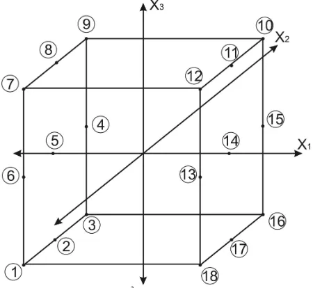
For this investigation, there were held a number of cuttings, which variables was based on the design of experiments methodology[25.26]. Eight experiments represent 23 factorial designs with added ten points in the middle edges and faces of the representation cube, Fig. 1, was taken. Taking into account three different levels for each variable, as shown in Table 1, there were taken the experimental conditions for 18 experiments, shown in Table 3.

TABLEI

UNITS FOR MAGNETIC PROPERTIES

Factor, coding (unit) Low (-1) Centre (0) High (1) Cutting speed, vc (m/min) 264 352 440 Feed, f (mm/rev) 0.06 0.08 0.12 Depth of cut, d (mm) 0.1 0.15 0.2

Fig 1. Representation of a 23 factorial design with added parameters

A. Workpiece and cutting tool material

The materials, which was manufactured in a CNC lathe OKUMA Lb 10II, was from AISI 316L steel, which hardness was 79HRB, as shown its properties in Table 2. Medically, the uses of stainless steels like 316L, although their high Fe contents render them non-compatible with magnetic resonance imaging (MRI) and to be poor fluoroscopic materials. In spite of their limitations and a myriad of materials have been chosen (like titanium), stainless steels are still favoured, as evidenced by the fact that seven out of the eight implants approved by the US Food and Drug Administration are made of stainless steels[27].

Regarding the use of coolants, 316L better results in tool wear and piece roughness are achieved when external coolant (emulsion 4–5% of a mineral oil in water) is used[28]. Furthermore, the development of new materials for cutting tools, such as TiN-coated cemented tungsten carbides, has also led to better control of the material removal process [29-31]

. Therefore, a coated tool from SECO specification: DNMG 110404 - M3 with TP 2000 coated grade was used for the manufacturing process. This has rhombic shape with cutting edge angle 55ο and are intended for general turning on steels and alloyed steels, as they are coated with four layers of Ti (C, N) + Al2O3 + Ti (C, N) + TiN. The rake angle mounted in the toolholder is γ-5ο and inclination angle is λs-9.5

ο

. The tool cutting edge angle is κ 93ο.

Small cylindrical parts with diameter 30mm and length 28mm with a conical hole were used to manufacture the spheres, femoral heads, Fig. 2.

TABLEII

MATERIAL PROPERTIES

Material Properties AISI 316L Stainless Steel Physical

Density 8 g/cc

Mechanical

Hardness, Rockwell B 79 Tensile Strength, Ultimate 560 MPa Tensile Strength, Yield 290 MPa Elongation of Break 50% Modulus of Elasticity 193 GPa Poisson ‘s Ratio 0.29

B. Measurements

During the procedure there were measured the forces that acted to the tool. For this reason a special device held a Kistler dynamometer 9257A, as shown in Fig. 2b. This is a three-component piezoelectric dynamometer platform. The force data were recorded by a specifically designed, very compact multi-channel microprocessor controlled data acquisition system with a single A/D converter preceded by a multiplexer. The results are recorded in Table 3.

C. Finite Elements Analysis

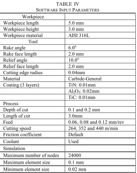
After the experiments, there were held a number of analyses according to the experimental conditions. Through AdvantEdge™ software there were all experiments run in simulation mode in order to predict the cutting forces and to compare the experimental results with the results from the analysis. The software inputs parameters are shown in Table 4.

V. RESULT AND DISCUSSION

TABLE IV

SOFTWARE INPUT PARAMETERS

Workpiece

Workpiece length 5.0 mm Workpiece height 3.0 mm Workpiece material AISI 316L

Tool

Rake angle 6.0ο Rake face length 2.0 mm Relief angle 10.0ο Relief face length 2.0 mm Cutting edge radius 0.04mm Material Carbide-General Coating (3 layers) TiN: 0.01mm

Al2O3: 0.02mm TiC: 0.01mm Process

Depth of cut 0.1 and 0.2 mm Length of cut 3.0mm

Feed 0.06, 0.08 and 0.12 mm/rev Cutting speed 264, 352 and 440 m/min Friction coefficient Default

Coolant Used

Simulation

Maximum number of nodes 24000 Maximum element size 0.1 mm Minimum element size 0.02 mm

If there is a comparison between the results in order to find the error, it will be two pairs, the error between numerical and experimental values and the error between predicted and experimental values. The errors can be found using the following formulas:

% 100 Pr

x alvalue

Experiment

ue edictedval alvalue

Experiment

Error = −

From the comparison of the values it is exported that the error is not grater than 11.5% for the majority of the experiments. There are two values which have error 16.5% and 31.5%. For this two pair it can be concluded that there were a mistake during the procedure or a measurement fault, something which affect the result. For all the others the different is normal, because with the Finite Element analysis which is predicted the values there will be an error less than 15%. A clear view of these results it can be exported from the graphs below, Fig. 3 and 4, where there the results for the two cutting depth, 01 and 0.2mm.

Fig. 3 Comparison of cutting forces between experimental and predicted values for cutting depth of 0.2mm

Fig. 4 Comparison of cutting forces between experimental and predicted values for cutting depth of 0.1mm

In order to compare better the results of the two methods, numerical and experimental an analysis of variance (ANOVA) was held between the forces and the cutting parameters separately for each method. The variation between the groups of cutting parameters represents systematic variation due to the effect on the forces. The between-groups variation is often called the effect variance and the within-groups variance is often called the error variance. In statistical terms, the analysis will tell whether the groups differ significantly or not. If a result is statistically significant, it tells that the group means are too different to have been that way by chance alone. Two levels of significance, p<0.05 and p<0.01, are typically employed in statistics. These mean that the probability of getting that result alone is less than 5% and 1% perceptively. These give pretty good confidence that the result obtained is a true reflection of an actual difference [32,33]. Through this analysis, it was examined an important aspect of statistical modelling, which distinguishes it from mere function approximation, the interpretability of results [34]. In Table 5 it is shown the analysis of the experimental Forces and in Table 6 the analysis of predicted Forces.

TABLE V

ANOVA OF THE EXPERIMENTAL RESULTS

Source DF SS MS F P

Cutting Depth 1 4900.5 4900.5 53.10 0.000 Cutting Speed 2 1834.8 917.4 9.94 0.003 Feed rate 2 7057.4 3258.7 38.23 0.000 Error 12 1107.6 92.3

Total 17 14900.3

S = 9.60710 R2 _{= 92.57% R}2_{(adj) = 89.47%}

TABLE VI

ANOVA OF THE PREDICTED RESULTS

Source DF SS MS F P

Cutting Depth 1 4933.6 4933.6 67.61 0.000 Cutting Speed 2 1309.8 654.9 8.15 0.006 Feed rate 2 4333.4 2166.7 26.69 0.000 Error 12 875.7 73.0

Total 17 11452.4

S = 8.5423 R2 = 92.35% R2(adj) = 89.17%

ones, the F-value for cutting speed is the same for both of them. Hence all three analyses are found to be adequate.

In Figure 5 there is the comparison of the distribution of temperature and chip between four analyses, with the first 440m/min cutting speed, 0.06 mm/rev feed rate and 0.2 cutting depth at position of 60ο, the second with 264m/min cutting speed, 0.06 mm/rev feed rate and 0.2 cutting depth at position of 9ο, the third 352m/min cutting speed, 0.08 mm/rev feed rate and 0.2 cutting depth at position of 30ο and the forth with 440m/min cutting speed, 0.12 mm/rev feed rate and 0.1 cutting depth at position of 9ο.

From this comparison it can be seen the form of the chip that is produced, when the cutting speed and feed rate changes.

Fig. 5 Distribution of temperature and chip between (a) 440m/min cutting speed, 0.06 mm/rev feed rate and 0.2 cutting depth at position of 60ο_{, (b)} with 264m/min cutting speed, 0.06 mm/rev feed rate and 0.2 cutting depth

at position of 9ο, (c) 352m/min cutting speed, 0.08 mm/rev feed rate and 0.2 cutting depth at position of 30ο and (d) with 440m/min cutting speed,

0.12 mm/rev feed rate and 0.1 cutting depth at position of 9ο

As it can be seen also, the values of the forces are decreasing as the cutting speed increases and the cutting depth and feed rate is decreasing. The highest decrease was for cutting speed of 352m/min, where for the same depth and feed rate, there were at about 25% decrease. For cutting speed 440m/min the amount of change was smaller. The effect of cutting speed can be attributed to the fact that as speed decreases, the shear angle decreases and the friction coefficient increases. Both effects increase the cutting force[35]. From the other hand the increase of cutting depth and feed rate, increases the amount of the removed material, so is increasing the resistance to the tool, which means the increase of the cutting speed. To this increase, it can be outputted that the cutting depth affects the forces directly proportional as it quite double, when the depth is twice increased. However the proportion of the feed rate is not direct, according to the results, which lead to the choice of the k2 factor in the numerical model.

So in these experiments, the forces for the manufacturing with cutting speed 440m/min, cutting depth 0.1mm and feed rate 0.06mm/rev are the smallest from all. So in these conditions it can be made easier and with less tool wear the manufacturing of the spheres of femoral heads. As the feed rate becomes bigger up to 0.12mm/rev the forces increases and with the cutting depth the relevance between them is proportional. The highest cutting force were logically

at 264m/min cutting speed with cutting depth 0.2mm and feed rate 0.12mm/rev, and its value 129N.

Surface roughness

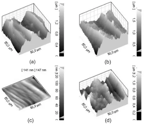
To fully characterize the process quality, all balls were measured after their fabrication in an Atomic Force Microscope (AFM). This technique was used for two reasons. Firstly, we have to measure very low and accurate values of roughness, and secondly, it is a quite good method for measuring spherical surfaces, as it can measure a very small surface, i.e., 50 x 50 µm, considering it as a flat portion of the sphere. It was found that the surface quality becomes better as the cutting speed increases. The surface roughness was predicted by measuring at five points of each sphere. Each measure was revised three times, in order to eliminate the fault factor. This procedure was repeated for a number of places along the profile, where the heights of lays and feed marks variation play a significant role for surface quality. The results of four measures, as they have been taken from the software of the AFM, are shown in Fig 6.

Fig. 6: Surface topography of manufactured femoral heads (a) with 352m/min cutting speed, 0.06 mm/rev feed rate and 0.2mm cutting depth, (b) with 440m/min cutting speed, 0.06 mm/rev feed rate and 0.2mm cutting

depth, (c) with 440m/min cutting speed, 0.06 mm/rev feed rate and 0.1mm cutting depth, (d) with 352m/min cutting speed, 0.08 mm/rev feed rate and

0.1mm cutting depth

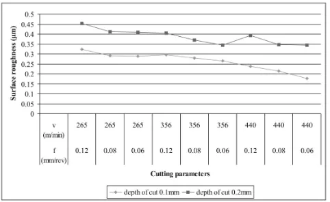
Fig. 7: Surface roughness for manufacturing spheres

VI. CONCLUSION

To summarize this paper refers to the forces that act on the tool during the manufacturing of femoral heads with high speed turning.

1. The predicted values from the finite element software in this investigation have a deflection not more than 12%.

2. The higher the cutting speed and lower cutting depth and feed rate the lower are the cutting forces that acts on the system tool and manufactured part.

3. The highest decrease was for cutting speed of 352m/min, where for the same depth and feed rate, there were at about 25%

4. Expansion of tool life, because small cutting forces cause less tool wear, and of course to better surface quality which plays a very important role to the manufacturing of femoral heads according to the strict regulations of ISO 7206.

5. An increase in tool life was throughout apparent due to small cutting forces and better surface quality. as the conclusion. A conclusion might elaborate on the importance of the work or suggest applications and extensions.

REFERENCES

[1] Ahmed N., Mitrofanov A.V., Babitsky V.I., Silberschmidt V.V., Analysis of forces in ultrasonically assisted turning. Journal of Sound and Vibration, 308, 2007, pp. 845–854

[2] Toenshoff H.K., Friemuth T., Andrae P., Lapp C., High speed cutting-fundamentals and machine tool development, 10th Int. Conf. on Precision Engineering, 2001, Yokohama, Japan

[3] Audy J., An appraisal of techniques and equipment for cutting force measurement. Journal of Zhejiang University SCIENCE A, 11, 2006, pp. 1781 – 1789

[4] Remadna M., Rigal J. F., Evolution during time of tool wear and cutting forces in the case of hard turning with CBN inserts. Journal of Materials Processing Technology, 178, 2006, pp. 67–75

[5] Tlusty G., Manufacturing process and equipment, Prentice Hall, New Jersy; 2000

[6] Trent E., Wright P., Metal Cutting, Butterworth-Heinemann, Oxford;2000

[7] Brinksmeier E., Mayr P., Lübben T., Pouteau P., Diersen P., Influence of Material properties on surface integrity and chip formation in high speed turning. 3rd International Conference on Metal Cutting and High Speed Machining, 2001, Metz, France

[8] Buck K. E., Scharpf D. W., Stein E. and Wunderlich W., Finite Elemente in der Statik. Verlag von Wilhelm Ernst & Sohn, Berlin – München – Düsseldorf, 1973

[9] Huebner K. H., The Finite Element Method for Engineers. John Wiley and Sons, New York – London – Sydney – Toronto, 1975

[10] Chandrupatla T. R., Belegundu A. D., Introduction to Finite Elements in Engineering. Prentice – Hall International Editions, New Jersey,

[11] Shih A. J., Finite element analysis of the rake angle effects in orthogonal metal cutting, Int. J. Mech. Sci., 38/1, 1996, pp. 1-17 [12]Carroll J. T. III, Strenkowsk J. S., Finite element models of orthogonal

cutting with application to single point diamond turning, Int. J. Mech. Sci., 30/12, 1988, pp. 899-920

[13]Xie J.Q., Bayoumi A.E., Zbib H.M., FEA modeling and simulation of shear localized chip formation in metal cutting, International Journal of Machine Tools & Manufacture, 38, 1998, pp.1067–1087

[14]Fang G., Zeng P., Three-dimensional thermo–elastic–plastic coupled FEM simulations for metal oblique cutting processes, Journal of Materials Processing Technology, 168, 2005, pp. 42–48

[15]Uhlmann E., Graf M., Zettier R., Finite Element Modeling and Cutting Simulation of Inconel 718, Annals of the CIRP, 56/1, 2007, pp. 61-64 [16]Zhang L., On the separation criteria in the simulation of orthogonal metal cutting using the finite element method, Journal of Materials Processing Technology, 89–90, 1999, pp. 273–278

[17]Baeker M., Roesler J., Siemers C., A finite element model of high speed metal cutting with adiabatic shearing, Computers and Structures, 80, 2002, pp. 495–513

[18]Kose E., Kurt A., Seker U., The effects of the feed rate on the cutting tool stresses in machining of Inconel 718, Journal of Materials Processing Technology, 196, 2008, pp. 165–173

[19]Yen Y.-C., Söhner J., Lilly B., Altan T., Estimation of tool wear in orthogonal cutting using the finite element analysis, Journal of Materials Processing Technology, 146, 2004, pp. 82–91

[20]Hashimura M., Ueda K., Dornfeld D., Manabe K., Analysis of Three-Dimensional Burr Formation in Oblique Cutting, Annals of the ClRP, 44/1, 1995, pp. 27-30

[21]Mouazen A. M., Nemenyi M., Finite element analysis of subsoiler cutting in non-homogeneous sandy loam soil, Soil & Tillage Research, 51, 1999, pp. 1-15

[22]Bil Η., S. Kilic S. E., Tekkaya A. E., A comparison of orthogonal cutting data from experiments with three different finite element models, International Journal of Machine Tools & Manufacture, 44, 2004, pp. 933–944

[23]Baeker M., Finite element simulation of high-speed cutting forces, Journal of Materials Processing Technology, 176, 2006, pp. 117–126 [24]Davim J. P., Maranhγo C., 2009. A study of plastic strain and plastic

strain rate in machining of steel AISI 1045 using FEM analysis. Materials and Design, 30: 160–165

[25]Dabnun M. A., Hashmi M. S. J., El-Baradie M. A., 2005. Surface roughness prediction model by design of experiments for turning machinable glass–ceramic (Macor), Journal of Materials Processing Technology, 164–165, 2005, pp. 1289–1293.

[26]Ross P. J., 1996. Taguchi techniques for quality engineering, Mc Graw-Hill, New York

[27]Lo K. H., Shek C. H., Lai J. K. L., Recent developments in stainless steels, Materials Science and Engineering R, 65, 2009, pp. 39 – 104 [28]Gandarias A., López de Lacalle L. N., Aizpitarte X., Lamikiz A., Study

of the performance of the turning and drilling of austenitic stainless steels using two coolant techniques, International Journal Machining and Machinability of Materials, Vol. 3, No. 1/2, 2008, pp. 1–17. [29]M’ Saoubi R., Outeiro J. C., Changeux B., Lebrun J. L., Morao Dias

A., Residual stress analysis in orthogonal machining of standard and resulfurized AISI 316L steels, Journal of Materils Processing Technology, 96, 1999, pp. 225 – 233

[30]Outeiro J. C., Umbrello D., M’ Saoubi R., Experimental and numerical modelling of the residual stresses induced in orthogonal cutting of AISI 316L steel, International Journal of Machine Tools & Manufacture, 46, 2006, pp. 1786 – 1794

[31]Umbrello D., M’ Saoubi R., Outeiro J. C., The influence of Johnson– Cook material constants on finite element simulation of machining of AISI 316L steel, International Journal of Machine Tools & Manufacture, 47, 2007, pp. 462 – 470

[32] Turner J. R., Thayer J. F., Introduction to analysis of Variance, Sage Publication Inc., California, 2001

[33]Hinkelmann K., O.Kempthorne O., Design and Analysis of Experiments, John Wiley & Sons, Inc., Canada, 1994

[34] Schimek M. G., Smoothing and Regression – Approaches, Computation and Application, John Willey and Sons, Canada, 2000 [35]Kalpakjian S., Manufacturing Processes for Engineering Materials,

Addison Wisley Longman Inc., Canada, 1997

[36]Galanis N. I., Manolakos D. E., Surface roughness of manufactured femoral heads with high speed turning, Int. J. Machining and Machinability of Materials, Vol. 5, No. 4, 2009, pp.371–382 [37]Galanis N. I., Manolakos D. E., Surface roughness prediction in