Analysis of Software Project Reports for Defect
Prediction Using KNN
Rajni Jindal, Ruchika Malhotra and Abha Jain
Abstract— Defect severity assessment is highly essential for the software practitioners so that they can focus their attention and resources on the defects having a higher priority than the other defects. This would directly impact resource allocation and planning of subsequent defect fixing activities. In this paper, we intend to predict a model which will be used to assign a severity level to each of the defect found during testing. The model is based on text mining and machine learning technique. We have used KNN machine learning method to predict the model employed on an open source NASA dataset available in the PITS database. Area Under the Curve (AUC) obtained from Receiver Operating Characteristics (ROC) analysis is used as the performance measure to validate and analyze the results. The obtained results show that the performance of KNN technique is exceptionally well in predicting the defects corresponding to top 100 words for all the severity levels. Its performance is less for top 5 words, better for top 25 words and still better for top 50 words. Hence, with these results, it is reasonable to claim that the performance of KNN is dependent on the number of words selected as independent features. As the number of words increases, the performance of KNN also gets better. Apart from this, it has been noted that KNN method works best for medium severity defects as compared to the other severity defects.
Index Terms—Receiver Operating Characteristics, Text mining, Machine Learning, Defect, Severity, K-Nearest Neighbour
I. INTRODUCTION
Now-a-days, various defect reporting/ tracking systems such as Bugzilla, CVS etc. are maintained for open source software repositories. These systems play an important role in tracking the defects which may be introduced in the source code [14]. These defects are then reported in a defect management system (DMS) for further analysis. Although, the issues of software are tracked using defect tracking systems which store the reported defects along with their details.
However, the data present in such systems is generally in unstructured form. Hence, text mining techniques in combination with machine learning techniques are required to analyze the data present in the defect tracking system.
Manuscript received March 14, 2014; March 31, 2014 Prof. Rajni Jindal is with Indira Gandhi Delhi Technical
University for Women, Delhi, India (email: [email protected]) Dr. Ruchika Malhotra (Corresponding Author phone: 91-011-26431421) is with Delhi Technological University, Delhi, India (email:
Abha Jain is with Delhi Technological University, Delhi, India (email: [email protected])
In the present scenario, an automated tool is required to collect the data from software repositories so that it can be analyzed and interpreted in order to make generalized conclusions. The defects in the software may be associated with various severity levels. For instance, catastrophic defects are the most severe defects and a failure caused by such defects may lead to a whole system crash [1], [5].
In this paper, we mine the information from the NASA’s database called PITS (Project and Issue Tracking System), by developing a tool that will first extract the relevant information from PITS using text mining techniques. After extraction, the tool will then predict the defect severities using machine learning techniques. The defects are classified into five categories of severity by NASA’s engineers as very high, high, medium, low and very low. In this work, we have used K-nearest neighbor (KNN) technique to predict the defects at various levels of severity. The prediction of defect severity will help the researchers and software practitioners to allocate their testing resources on more severe areas of the software. The performance of the predicted model will be analyzed using Area Under the Curve (AUC) obtained from Receiver Operating Characteristics (ROC) analysis.
The rest of this paper is organized as follows: Section 2 reviews the key points of available literature in the domain. Section 3 describes the research method used for this study, which includes the data source and model evaluation criteria. Section 4 presents the result analysis. Section 5 concludes the paper and outlines directions for future work.
II. LITERATURE REVIEW
for software defect prediction i.e. for predicting whether a particular part of the software is defective or not. A very effective tool based on Natural Language Processing
(NLP) was developed by Runeson et al. [18] and Wang et al. [22] that was used to detect duplicate reports. Cubranic and Murphy [4] analyzed an incoming bug report and proposed an automated method that would assist in bug triage to predict the developer that would work on the bug based on the bug description. Canfora and Cerulo [3] discussed how software repositories can help developers in managing a new change request, either a bug or an enhancement feature. Also, a lot of empirical work has been carried out in predicting the fault proneness of classes in object-oriented (OO) software systems using a number of OO design metrics [2], [5], [7], [8], [11], [12], [15], [16], [23], [25]. Although, these studies were based on finding the relationship between OO metrics and fault proneness of classes, but did not focus on the severity of faults. Till date, there are only a few studies which were based on finding the relationship between OO metrics and fault proneness of classes at different levels of severity of faults. The most efficient work in the field of fault severity has been done by the authors Singh et al. [21]. They have analyzed the performance of models at high, medium and low severity faults and found that the model predicted at high severity faults has lower accuracy than the models predicted at medium and low severities. The validation of the proposed models was done using various OO metrics like CBO, WMC, RFC, SLOC, LCOM, NOC, DIT on the public domain NASA dataset KC1 using DT and ANN as the machine learning methods and LR as the statistical method. The conclusion drawn was that DT and ANN models outperformed the LR model and that CBO, WMC, RFC and SLOC metrics are significant across all severity of faults and DIT metric is not significant across any severity of faults. LCOM and NOC are not found to be significant with respect to LSF. Somewhat same results were also concluded in the paper by Zhou and Leung [24]. They have investigated the fault-proneness prediction performance of OO design metrics with regard to ungraded, high, and low severity faults by employing statistical (LR) and machine learning (Naïve Bayes, Random Forest, and NNge) methods. From both the above papers, it was summarized that the design metrics are able to predict low severity faults in fault-prone classes better than high severity faults in fault-fault-prone classes. Bayesian approach was also used by the author Pai [17] in his work to find the relationship between software product metrics and fault proneness. Shatnawi and Li [20] focused on identifying error-prone classes in post-release software evolution process. They studied the effectiveness of software metrics and examined three releases of the Eclipse project. They observed that, the accuracy of the prediction decreased from release to release and that there are only a few metrics which can predict class proneness in three error- severity categories.
The work proposed in this paper is similar to the work done by Menzies and Marcus [13]. The authors have presented an automated method named SEVERIS (SEVERity Issue assessment) which is used to assign severity levels to the defect reports by using the data from NASA’s Project and Issue Tracking System (PITS). Their method is based on the automated extraction and analysis of textual descriptions from issue reports in PITS by using various text mining techniques.
They have used a rule learning method as their classification method to assign the features with proper severity levels, based on the classification of the existing reports. Similar work has also been done by Sari and Siahaan [19]. They have also developed a model for the assignment of the bug severity level. They have used the same pre-processing tasks (tokenization, stop words removal and stemming) and feature selection method (InfoGain), but, have used SVM as their classification method. Lamkanfi et al. [10] have also analyzed the textual description using text mining algorithms in order to propose a technique that is used to predict the severity of a reported bug against three open – source projects viz. Mozilla, Eclipse and GNOME using Bugzilla as their bug tracking system and Naïve Bayes as their classifier.
III. RESEARCH METHODOLOGY
In this section, we present our research method. We first introduce the data source which elaborates on the dataset being used in our study followed by the text classification framework that we have used in order to extract the relevant words from the defect descriptions. Finally, we describe our model evaluation criteria.
A. Data Source
We have collected the defect data from an open source NASA’s dataset called PITS (Project and Issue Tracking System). There are various projects that come under PITS database all of which were supplied by NASA’s Software Verification and Validation (IV & V) Program. We have used PITS B project wherein the data has been collected for more than 10 years and includes all the issues that have been found in the robotic satellite missions and human rated system. The focus of our study is to investigate the predictiveness of the model with regard to the severity of defects. Therefore, we are interested in the number of defects at each severity level as shown in Table I.
NASA’s engineers have classified severity 1 defects as Very High, severity 2 defects as High, severity 3 defects as Medium, severity 4 defects as Low and severity 5 defects as Very Low. We are interested only in the last four severity levels i.e. severity 2, severity 3, severity 4 and severity 5 as it can be seen from table 1 that there are no severity one issues in the defect data. This is so because these defects are of very high severity level and therefore possibility of such defects in the software become very rare.
Hence, we applied different methods of text mining for dimensionality reduction in the following order: tokenization, stop word removal, stemming, feature selection and weighting.
TABLE I. NUMBER OF DEFECT REPORTS OF PITSBDATASET AT
EACH SEVERITY LEVEL
Severity 1 Severity 2 Severity 3 Severity 4 Severity 5
Pits B 0 23 523 382 59
1)Pre-processing
Pre-processing is the first and foremost step of text mining which is done in order to remove the irrelevant words from the document. Irrelevant words are the words which are not important for the learning task and rather their usage can substantially degrade performance of machine learning methods. The three most popular methods which are used for pre-processing are tokenization, stop words removal and stemming. Tokenization is the process of converting a stream of characters into a sequence of tokens. We have done tokenization by replacing the punctuation with blank spaces, removing all the non-printable escape characters and converting all the words to lowercases. Thereafter, all the stop words like prepositions, conjunctions, articles, common verbs, nouns, pronouns, adverbs and adjectives were removed from the dataset by using a list of English stop words. Finally, stemming was performed which removes words with the same stem and keeps the stem as the feature. For example, the words “train”, “training”, “trainer” and “trains” can be replaced with “train”. All the words obtained after preprocessing were called as ‘features’.
2)Feature selection
Even after performing a series of pre-processing tasks, the
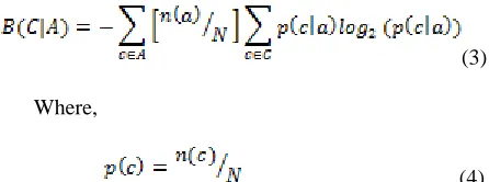
number of words in the document can still be very large. Therefore, feature selection method is used in order to further reduce the dimensionality of the feature set. There are a number of such methods available in the literature like document frequency, term frequency, mutual information, information gain, odds ratio, χ2statistic, term strength etc. These methods use an evaluation function that is applied to a single word. Thereafter, all these words are ranked by their independently determined scores, and then the top scoring words are selected.In this paper, InfoGain measure is used to rank all the features obtained after pre-processing and then the top ‘N’ scoring features are selected based on the rank. According to the InfoGain measure, the best words are those that most simplifies the target concept, which is in our case, the distribution of severities [13]. Suppose a data set has 80% severity=5 issues and 20% severity=1 issues. Then that data set has a class distribution C0with classes c(1) = severity5and
c(2) = severity1 with frequencies n(1) = 0.8 and n(2) = 0.2. The number of bits required to encode an arbitrary class distribution C0is B(C0) defined as follows:
(1) Where,
(2)
If A is a set of attributes, then the number of bits required to encode a class after observing an attribute is:
(3)
Where,
(4) The highest ranked attribute Ai is the one with the largest information gain; i.e., the one that most reduces the encoding required for the data after using that attribute; i.e.
(5)
3)Weighting and Normalizing
Now, these ‘N’ features can be represented as t1, t2, . . . , tN.
The ith document is then represented as an ordered set of N
values, called an N-dimensional vector which is written as (Xi1, Xi2, . . . , XiN ) where Xij is a weight measuring the
importance of the jth term tjin the ith document. The complete
set of vectors for all documents under consideration is called a vector space modelor VSM.
There are various methods which can be used for weighting the terms. We have used TFIDF approach for calculating the weights, which stands for Term Frequency Inverse Document Frequency. Term frequency is simply the frequency of the jth term, i.e. tj, in document i. This value makes the terms that are
frequent in the given document more important than the others. The second value i.e. inverse document frequency is given by log (n/nj) where nj is the number of documents
containing term tj and n is the total number of documents. This
value makes the terms that are rare across the collection of documents more important than the others.
Now, before we use the set of N-dimensional vectors, we will first need to normalize the values of the weights. It has been observed that ‘normalizing’ the feature vectors before submitting them to the learning algorithm is the most necessary and important condition.
B. Model Evaluation
As we all know, defect-prone documents are treated as the positive instances in the context of defect prediction [9]. On this basis, we can categorize the defect prediction results into four different types as defined below:
- FN (False Negative): defect-prone documents that are wrongly classified to be defect- free;
- TN (True Negative): defect-free documents that are classified correctly;
- FP (False Positive): defect-free documents that are wrongly classified to be defect-prone.
To measure the performance of the predicted model, we have used the following performance evaluation measures:
1) Sensitivity
It measures the correctness of the predicted model and is defined as the percentage of the documents correctly predicted to be defect prone. It is also referred to as Recall. Mathematically we can define sensitivity as,
(6)
2) Receiver Operating Characteristics (ROC) analysis ROC curve is defined as a plot of sensitivity on the y-
coordinate versus its 1-specificity on the x- coordinates [6]. The main objective of constructing ROC curves is to obtain the required optimal cut-off point that maximizes both sensitivity and specificity. An overall indication of the accuracy of a ROC curve is the area under the curve (AUC). Values of AUC range from 0 to 1 and higher values indicate better prediction results.
3) Validation method used
The validation method used in our study is Hold-out validation (70-30 ratio) in which the entire dataset is divided into 70% training data and remaining 30% as test data. There are two methods by which we can assign the cases. Either we can randomly assign the cases based on relative number of cases or else we can use a partitioning variable. We have not randomly assigned the cases, but have rather used a partitioning variable to assign the cases. In other words, we have used a variable that splits the given dataset into training and testing samples in 70-30 ratio. This variable can have the value either 1 or 0. All the cases with the value of 1 for the variable are assigned to the training samples and all the other cases are assigned to the testing samples.
To get more generalized and accurate results, we have done validation using 10 separate partitioning variables. A single variable is used at a time on the basis of which the given dataset will be divided randomly in the ratio of 70-30. The corresponding training samples will be used by KNN in order to predict the model and the remaining testing samples will be used to validate the model. The same process is repeated for 10 runs corresponding to each partitioning variable.
IV. RESULT ANALYSIS
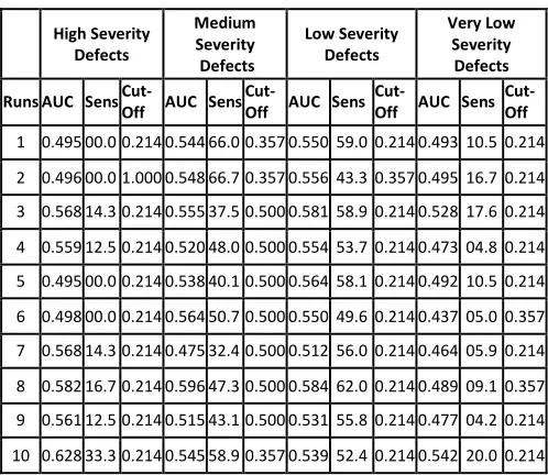
[image:4.612.312.561.159.375.2]In this section, we have analyzed the results corresponding to the top-5, 25, 50 and 100 words in order to predict the best model that gives the highest accuracy using sensitivity, AUC and the cut-off point as the performance measures. Tables II- V present and summarize the results with respect to high, medium, low and very low severity levels.
TABLE II. RESULTS OF KNNFOR TOP-5WORDS
High Severity Defects
Medium Severity Defects
Low Severity Defects
Very Low Severity Defects
Runs AUC Sens
Cut-Off AUC Sens
Cut-Off AUC Sens
Cut-Off AUC Sens Cut-Off
1 0.495 00.0 0.214 0.544 66.0 0.357 0.550 59.0 0.214 0.493 10.5 0.214
2 0.496 00.0 1.000 0.548 66.7 0.357 0.556 43.3 0.357 0.495 16.7 0.214
3 0.568 14.3 0.214 0.555 37.5 0.500 0.581 58.9 0.214 0.528 17.6 0.214
4 0.559 12.5 0.214 0.520 48.0 0.500 0.554 53.7 0.214 0.473 04.8 0.214
5 0.495 00.0 0.214 0.538 40.1 0.500 0.564 58.1 0.214 0.492 10.5 0.214
6 0.498 00.0 0.214 0.564 50.7 0.500 0.550 49.6 0.214 0.437 05.0 0.357
7 0.568 14.3 0.214 0.475 32.4 0.500 0.512 56.0 0.214 0.464 05.9 0.214
8 0.582 16.7 0.214 0.596 47.3 0.500 0.584 62.0 0.214 0.489 09.1 0.357
9 0.561 12.5 0.214 0.515 43.1 0.500 0.531 55.8 0.214 0.477 04.2 0.214
10 0.628 33.3 0.214 0.545 58.9 0.357 0.539 52.4 0.214 0.542 20.0 0.214
TABLEIII. RESULTS OF KNNFOR TOP-25WORDS
High Severity Defects Medium Severity Defects Low Severity Defects Severity Defects Very Low
Runs AUC Sens
Cut-Off AUC Sens
Cut-Off AUC Sens
Cut-Off AUC Sens
Cut-Off
1 0.596 25.0 0.214 0.708 70.1 0.357 0.646 39.3 0.357 0.533 21.1 0.214
2 0.691 40.0 0.214 0.739 73.7 0.357 0.697 48.6 0.357 0.595 33.3 0.214
3 0.620 28.6 0.214 0.682 69.4 0.357 0.650 46.8 0.357 0.548 23.5 0.214
4 0.795 62.5 0.214 0.726 71.1 0.357 0.669 51.2 0.357 0.587 28.6 0.214
5 0.659 33.3 0.214 0.729 70.4 0.357 0.681 51.3 0.357 0.566 26.3 0.214
6 0.684 40.0 0.214 0.696 70.9 0.357 0.653 51.3 0.357 0.632 40.0 0.214
7 0.701 42.9 0.214 0.690 69.9 0.357 0.666 45.7 0.357 0.575 29.4 0.214
8 0.590 20.0 0.214 0.708 63.2 0.357 0.639 49.6 0.357 0.530 25.0 0.214
9 0.699 44.4 0.214 0.754 71.4 0.357 0.692 51.6 0.357 0.567 25.0 0.214
10 0.822 66.7 0.214 0.738 67.4 0.357 0.677 50.9 0.357 0.573 25.0 0.214
TABLEIV. RESULTS OF KNNFOR TOP-50WORDS
High Severity Defects Medium Severity Defects Low Severity Defects Severity Defects Very Low
Runs AUC Sens
Cut-Off AUC Sens
Cut-Off AUC Sens
Cut-Off AUC Sens
[image:4.612.313.567.426.643.2]1 0.698 50.0 0.214 0.746 70.7 0.357 0.709 49.6 0.357 0.701 52.6 0.214
2 0.678 40.0 0.214 0.762 73.0 0.357 0.762 57.9 0.357 0.663 44.4 0.214
3 0.682 42.9 0.214 0.758 65.0 0.357 0.668 47.6 0.357 0.674 52.9 0.214
4 0.582 25.0 0.214 0.798 75.0 0.357 0.739 47.2 0.357 0.834 76.2 0.214
5 0.813 66.7 0.214 0.810 75.7 0.357 0.757 54.7 0.357 0.681 47.4 0.214
6 0.632 30.0 0.214 0.754 70.9 0.357 0.697 53.0 0.357 0.712 55.0 0.214
7 0.754 57.1 0.214 0.796 71.0 0.357 0.739 58.6 0.357 0.675 47.1 0.214
8 0.564 20.0 0.214 0.748 70.1 0.357 0.708 53.8 0.357 0.660 50.0 0.214
9 0.742 55.6 0.214 0.728 67.9 0.357 0.681 50.8 0.357 0.562 25.0 0.214
10 0.648 33.3 0.214 0.759 70.2 0.357 0.670 57.3 0.357 0.721 55.0 0.214
TABLEV. RESULTS OF KNNFOR TOP-100WORDS
High Severity Defects Medium Severity Defects Low Severity Defects Very Low Severity Defects
Runs AUC Sens
Cut-Off AUC Sens
Cut-Off AUC Sens
Cut-Off AUC Sens
Cut-Off
1 0.734 50.0 0.214 0.751 72.1 0.357 0.698 54.7 0.366 0.713 57.9 0.214
2 0.687 40.0 0.214 0.779 67.8 0.357 0.749 60.7 0.357 0.665 50.0 0.214
3 0.692 42.9 0.214 0.775 72.5 0.357 0.710 86.3 0.214 0.705 58.8 0.214
4 0.610 25.0 0.214 0.785 75.0 0.357 0.699 50.4 0.357 0.813 76.2 0.214
5 0.822 66.7 0.214 0.795 78.3 0.357 0.724 49.6 0.357 0.680 47.4 0.214
6 0.689 40.0 0.214 0.749 70.3 0.357 0.675 77.4 0.214 0.707 50.5 0.214
7 0.775 57.1 0.214 0.781 75.0 0.357 0.721 55.2 0.357 0.638 41.2 0.214
8 0.732 50.0 0.214 0.778 74.7 0.357 0.722 51.2 0.357 0.547 27.3 0.214
9 0.732 50.0 0.214 0.760 72.2 0.357 0.708 54.9 0.357 0.600 41.7 0.214
10 0.732 50.0 0.214 0.776 67.4 0.357 0.742 65.7 0.357 0.716 53.3 0.214
From table II, it becomes clear that the performance of the model is consistent for all the severity levels when AUC is considered for evaluation. This is so because the values of AUC lie in the range of 0.4 to 0.6 for all the 10 consecutive runs, irrespective of the severity levels. However, there is a huge difference in the model prediction if we look at the sensitivity column. The maximum value of sensitivity for medium and low severity level is 66.7%, whereas its maximum value corresponding to high and very low severity level is just 33.3%. This trend suggests that model can predict medium severity defects better than the defects having either high or very low severity level when the number of words is less. As we increase the number of words to 25, we can see from table III that the prediction capability of the model is again the best for the medium severity defects with AUC in the range of 0.68 to 0.74 and is worst for very low severity defects with the maximum value of AUC being 0.6. Also, the sensitivity values for very low severity defects are just in the range of 21.1% to 40.0%. This trend is suggesting that there should be maximum focus on the defects having medium
severity level when the number of words considered is nominal.
A similar kind of trend can be seen from table IV, where the model has performed exceptionally well in predicting the medium severity defects as values for both AUC and sensitivity are highest as compared to other severity levels. But, it is evident from table V, that performance of the model is consistent with respect to all the four severity levels when considering AUC as the performance evaluation measure. However, the sensitivity values indicate that the model predicted with respect to medium and low severity defects should be preferred over the model predicted with respect to high and very low severity defects.
But if we compare the performance of the model in terms of the number of words considered for model prediction, then there is a very clear indication of the fact that the model performs exceptionally well when top 100 words were considered, and that its performance drastically reduces when the number of words considered for classification is less. Performance of the model is worst when top 5 words were taken into account, is still better for top 25 and 50 words, and best for top 100 words. Hence, with these results, it is reasonable to claim that the performance of KNN is dependent on the number of words selected as independent features. As the number of words increases, the performance of KNN also improves. Apart from this, we have also observed that KNN method works best for medium severity defects as compared to the other severity defects.
V. CONCLUSION
Due to the widespread use of open source software repositories, the use of defect tracking systems has become inevitable. The issues of the software are tracked using such systems which store the defects along with their details. Such defects introduced in the software may be of varying severity levels ranging from mild to catastrophic. Thus, defect tracking systems play an important role to capture the defect data. However, a common issue in such systems is that they are useful for storing day-to-day information. Moreover, the information contained within such systems is generally of unstructured form.
that KNN method works best for medium severity defects as compared to the other severity defects.
Although we analyzed only one project of PITS in our study so far, we believe that the research results can be generalized to the other projects available in the PITS database. So, our future work involves replication of this work in other projects of PITS.
REFERENCES
[1] K.K. Aggarwal, Y. Singh, A. Kaur and R. Malhotra, “Empirical analysis for investigating the effect of object-oriented metrics on fault proneness: A replicated case study,” Software Process: Improvement and Practice, vol. 16, no.1, pp. 39-62, 2009.
[2] C. Catal and B. Diri, “A systematic review of software fault prediction studies,” Expert Systems with Applications,vol.36, pp. 7346-7354, 2009. [3] G. Canfora and L. Cerulo, “How Software Repositories can Help in
Resolving a New Change Request,” Workshop on Empirical Studies in Reverse Engineering, 2005.
[4] D. Cubranic and G.C. Murphy, “Automatic bug triage using text categorization,” Proceedings of the Sixteenth International Conference on Software Engineering and Knowledge Engineering, 2004.
[5] K.E. Emam and W. Melo, “The Prediction of Faulty Classes Using Object-Oriented Design Metrics,” Technical report: NRC 43609, 1999. [6] K.E. Emam, S. Benlarbi, N. Goel and S. Rai, “A validation of
object-oriented metrics,” NRC Technical report ERB-1063, 1999.
[7] I. Gondra, “Applying machine learning to software fault-proneness prediction,” The Journal of Systems and Software, vol.81, pp. 186-195, 2008.
[8] T. Gyimothy, R. Ferenc and I. Siket, “Empirical validation of object-oriented metrics on open source software for fault prediction,” IEEE Transactions on Software Engineering, vol.31, no.10, pp. 897-910, 2005. [9] Y. Jiang, B. Cukic and Y. Ma,“Techniques for evaluating fault prediction
models,” Empirical. Software. Engineering, vol.13, no. 15, pp. 561-595, 2008.
[10] A. Lamkanfi, D. Serge, E. Giger and B. Goethals, “Predicting the Severity of a Reported Bug,” 7th IEEE working conference on Mining
Software Repositories (MSR), pp. 1-10, 2010.
[11] R. Malhotra and Y. Singh, “On the Applicability of Machine Learning Techniques for Object- Oriented Software Fault Prediction,” Software Engineering: An International Journal, vol.1, no.1, pp. 24-37, 2011. [12] R. Malhotra and A. Jain, “Fault Prediction Using Statistical and Machine
Learning Methods for Improving Software Quality,” Journal of Information Processing Systems,vol. 8, no.2, pp. 241- 262, 2012. [13] T. Menzies and A. Marcus, “Automated Severity Assessment of Software
Defect Reports,” IEEE International Conference on Software Maintenance (ICSM), 2008.
[14] G. Myers, T. Badgett, T. Thomas and C. Sandler, “The Art of Software Testing,” second ed., John Wiley & Sons, Inc., Hoboken, NJ, 2004. [15] N. Ohlsson, M. Zhao, M and M. Helander , “Application of multivariate
analysis for software fault prediction,” Software Quality Journal, vol.7, pp.51-66, 1998.
[16] H. Olague, L. Etzkorn, S. Gholston and S. Quattlebaum, “Empirical validation of three software metrics suites to predict fault-proneness of object-oriented classes developed using highly iterative or agile software development processes,” IEEE Transactions on Software Engineering, vol.33, no.8, pp. 402-419, 2007.
[17] G. Pai, “Empirical analysis of software fault content and fault proneness using Bayesian methods,” IEEE Transactions on Software Engineering, vol. 33, no. 10, pp. 675-686, 2007.
[18] P. Runeson, M. Alexandersson and O. Nyholm, “Detection of Duplicate Defect Reports Using Natural Language Processing,” 29th IEEE
International Conference on Software Engineering (ICSE),pp. 499 – 508, 2007.
[19] G.I.P. Sari and D.O. Siahaan, “An attribute Selection For Severity level Determination According To The Support Vector Machine Classification Result,” Proceedings of The 1st International Conference
on Information Systems For Business Competitiveness (ICISBC), 2011. [20] R. Shatnawi and W. Li, “The effectiveness of software metrics in
identifying error-prone classes in post-release software evolution process,” The Journal of Systems and Software,vol. 81, pp. 1868-1882, 2008.
[21] Y. Singh, A. Kaur and R. Malhotra,“Empirical validation of object-oriented metrics for predicting fault proneness models,” Software Quality Journal, vol.18, pp. 3-35, 2010.
[22] X. Wang, L. Zhang, T. Xie, J. Anvik and J. Sun, “An Approach to Detecting Duplicate Bug Reports using Natural Language and Execution Information,” Association for Computing Machinery, 2008.
[23] P. Yu, T. Systa, and H. Muller, “Predicting fault-proneness using OO metrics: An industrial case study,” In Proceedings of Sixth European Conference on Software Maintenance and Reengineering, Budapest, Hungary, pp.99-107, 2002.
[24] Y. Zhou, and H. Leung,“Empirical Analysis of Object-Oriented Design Metrics for Predicting High and Low Severity Faults,” IEEE Transactions on Software Engineering, vol. 32, no. 10, pp. 771-789, 2006.