An investigation into statistical methods for analysing ordered categorical data

An investigation into statistical methods for analysing

ordered categorical data.

GRETTON, John D.

Available from Sheffield Hallam University Research Archive (SHURA) at:

http://shura.shu.ac.uk/19727/

This document is the author deposited version. You are advised to consult the

publisher's version if you wish to cite from it.

Published version

GRETTON, John D. (1998). An investigation into statistical methods for analysing

ordered categorical data. Masters, Sheffield Hallam University (United Kingdom)..

Copyright and re-use policy

REFERENCE

Fines are charged at 50p per hour

2 7 FEB 2002

H - o

2 6 APR 2002

AA2 it_

6 > v \

_ 6 JUN 2002

7.

ProQuest Number: 10697029

All rights reserved

INFORMATION TO ALL USERS

The quality of this reproduction is dependent upon the quality of the copy submitted.

In the unlikely event that the author did not send a com plete manuscript and there are missing pages, these will be noted. Also, if material had to be removed,

a note will indicate the deletion.

uest

ProQuest 10697029

Published by ProQuest LLC(2017). Copyright of the Dissertation is held by the Author.

All rights reserved.

This work is protected against unauthorized copying under Title 17, United States C ode Microform Edition © ProQuest LLC.

ProQuest LLC.

789 East Eisenhower Parkway P.O. Box 1346

An investigation into statistical methods

for analysing ordered categorical data

John D. Gretton

A thesis submitted in fulfilment of the requirements for the degree of

Master of Philosophy

October 1998

School of Computing and Management Sciences

Acknowledgements

I am sincerely grateful to my director of studies, Dr. Bekia Fosam, and my supervision team, Mike Grimsley, Eric Okell, Steve Wisher and Keith Jones, for their invaluable help and guidance

throughout the course of the research. I was never found wanting for contact with people with bigger and different shaped brains than mine. Thanks a lot you guys.

I am indebted to my Examiners Dr Richard Gadsden and Professor Ian Dunsmore for their effort in inspecting this thesis (it can’t have been enjoyable), and their attitude in allowing me to make amendments for re-examination without any hassle, when time and computing resources have been at a premium for me since starting full-time work.

Fond regards to the SSRC for all kinds of stuff, like contract work to give me some extra pennies, administration (and then some!) and generally just being friendly, helpful people.

Big ta’s to Simon Alexander for mending my computer when it went down on me, and lending me the portable PC on which a fair proportion of this thesis was written. Same to Errol and Homed, too.

Much appreciation to Christine Straker for sorting me out loads of lecturing work to help my bank balance, communication skills and confidence, and to boost my CV. Cheers for being my referee, and the chats also.

Much respect is due to my good friends (Al, Paresh, Bob, Ad, Marky B., Jay, Si, Doggy Dave, Justin, Emma, Shelley & Dips) for listening to me moan about how hard I thought my research was, and helping to take my mind off it from time to time, as well as badgering me to get the corrections done for 10 months. Cheers Ears.

Many thankyous to Darren and Jo for a new place to live and the much sought after portable PC with which to correct the original incorrectness in this thesis. Same goes to Jonathan Gorst for his PC and office space for round 2 in the correction procedure.

Summary

This investigation researches statistical methods for analysing ordered categorical data. Some standard descriptive and modelling procedures are described, and the data is analysed using a relatively new statistical package, CHAID, which is designed purely for categorical data analysis. The study is centered around the application o f the proportional odds and continuation odds models, to data obtained from a survey o f the opinions o f South Yorkshire Police staff (SSRC (1994)). Morale within the South Yorkshire Police is the factor o f interest, and is discussed in some detail. The two approaches o f proportional odds and continuation odds models are discussed critically. Dummy variables and scored levels are employed for the treatment o f ordinal variables. The effects o f these two methods o f coding ordinal data, on the results o f the analyses, are also compared and discussed. Methods o f assessing the goodness-of-fit o f ordinal models are discussed, and a modification to the guidelines for using a recently presented technique (Lipsitz et al (1996)) is suggested and applied. The proportional odds model is successfully applied. The implications from the models produced are that job satisfaction, communication, public view of the police, promotion issues and length

Contents

Chapter 1: Introduction

1

Sections

1.1: The research problem - General 1

1.2: Categorical and ordered categorical data 1

1.3: Rationale for regression models with an

ordinal response variable 3

1.4: The research problem - Application 7

1.5: Organisation o f the thesis 7

Chapter 2: Methodology

9

Sections

2.1: Relevant developments of the methodology 9

2.2: Exploratory analysis for categorical and ordinal data 11

2.2.1: Contingency tables 11

2.2.2: Independence between variables 12

2.2.3: CHAID 13

2.2.4: Odds and odds ratios IS

2.2.5: Odds ratios and ordinal data 19

2.2.6: Measures of association for ordinal data 22

2.3: Standard models modified for ordinal variables 25

2.3.1: Scoring the levels of ordinal variables 25

2.3.2: Loglinear modelling 27

2.3.3 : Logit modelling 31

2.3.4: The Binary Logistic model 33

2.3.4.1: Parameter estimation

for the binary logistic model 34

2.3.5: Interactions between explanatory covariates 35

36 37 39 43

46 47

53

55 56 60

61

2.5: Criteria for assessing model fit 62

2.5.1: Indicators of model adequacy 62

2.5.2: Goodness-of-fit statistics

introduced by Lipsitz et al (1996) 65

2.5.3: Modifications to the guidelines

for using Lipsitz et al (1996) 71

2.5.4: Diagnostic plotting 75

Chapter 3: The data and exploratory data analysis

76

Sections

3.1: The South Yorkshire Police data 76

3.1.1: The South Yorkshire Police staff survey 76

2.4.1: The Ordinal Logistic Regression model 2.4.2: The Stereotype Model

2.4.3: The proportional odds model

2.4.3.1: The proportional odds assumption 2.4.3.2: Parameter estimation

for the proportional odds model 2.4.4: The continuation odds model

2.4.4.1: The continuation odds model and survival analysis

2.4.4.2: The continuation odds model and Cox’s proportional hazards model 2.4.4.3: Fitting the continuation odds model 2.4.4.4: The continuation odds assumption 2.4.4.5: Parameter estimation

3.1.2: Background information

on the South Yorkshire Police 77

3.1.3: Morale and morale o f the South Yorkshire Police 80

3.1.4: Measures o f morale 82

3.1.5: Explanatory variables 8 5

3.2: Application o f CHAID to the South Yorkshire Police data 98

3.2.1: Variable selection 98

3.2.2: CHAID analysis o f the South Yorkshire Police data 99 3.2.2a: Respondent’s own morale

and predictors subset 1 99

3.2.2b: Respondent’s own morale

and predictors subset 2 107

3.2.2c: Respondent’s own morale

and predictors subset 3 113

3.2.2d: Colleagues’ perceived morale

and predictors subset 1 116

3.2.2e: Colleagues’ perceived morale

and predictors subset 2 121

3.2.2f: Colleagues’ perceived morale

and predictors subset 3 124

3.2.2g: Relative morale and predictors subset 1 127

3.2.2h: Relative morale and predictors subset 2 131

3.2.2i: Relative morale and predictors subset 3 133

3.2.3: Summary o f CHAID results 134

Chapter 4: Modelling morale within the South Yorkshire Police 135

Sections

4.1: Defining the dependent variable, morale 135

4.2: The proportional odds model

4.2.1: Modelling morale using dummy variables

for ordinal variables 136

4.3: Modelling morale using scored levels for ordinal variables 158

4.3.1: Modelling morale o f officers 163

4.3.2: Modelling morale o f civil staff 170

4.4: Comparison o f dummy variables and scored categories 176

4.5: The continuation odds model

and the South Yorkshire Police data 177

4.6: Discussion o f the proportional odds

and continuation odds assumptions 179

Chapter 5: Conclusion, discussion and further research

180

Sections

5.1: Conclusion and discussion 180

5.2: Ideas for further research 183

References

Chapter 1: Introduction

1.1: The research problem - General

There is a distinct shortage o f statistical methodologies that deal specifically with ordered categorical data. Methods that have been developed are not widely used to analyse ordinal data, more often techniques for analysing nominal or interval data are applied. Therefore, there is a need for greater understanding of how to treat ordinal data, and possibly greater accessibility o f ordinal methods. There is uncertainty about the interpretation o f some ordinal models, and ways to assess their goodness-of-fit.

This research is centered around the analysis of data with an ordinal response variable, and addresses the problems involved in analysing ordered categorical data. Ordinal data occurs when a categorical variable has an intrinsic ordering to its levels, so an underlying continuum is assumed. This type o f data is very common in market research and medical studies, among other areas, thus the need for definitive methodologies is important.

1.2: Categorical and ordered categorical data

Categorical data arise frequently in many areas o f research. A categorical variable is one where the measurement scale is a set of categories, e.g. political belief may be gauged as ‘liberal’, ‘moderate’ or ‘conservative’, or pain after an operation might have response categories o f ‘none’, ‘mild’ or ‘severe’.

Categorical variables which do have ordered levels are called ordinal. Examples o f these could be social class (upper, middle, lower), attitude towards legalisation o f abortion (strongly disapprove, disapprove, neither, approve, strongly approve) or diagnosis o f multiple sclerosis (certain, probable, unlikely, definitely not). The categories o f ordinal variables are clearly ordered, and in a lot o f cases one could assume some underlying continuous scale. Whilst absolute distances between levels are unknown, one can conclude that someone categorised as ‘mild’ is in less pain than a person categorised as ‘severe’, although a quantitative measure o f how much less pain the individual is in is realistically unobtainable. An interval variable is one which does have quantifiable distances between levels, e.g. income or age.

An ordinal data variable is one where there are distinct categories with a definite ordering. For example in medical research one might come across a pain response o f none, mild or severe, or in market research response to a statement may be gauged by a likert scale variable with categories strongly agree, agree, neither agree nor disagree, disagree or strongly disagree. Both these examples assume an underlying continuous scale. The absolute distances between categories are not easily determinable, in that although no pain is better than mild or severe pain, and similarly mild pain is more favourable than severe pain, we cannot quantify precisely how much better. Similarly, whilst agreement or strong agreement with a statement may be desired, in the context o f some research, one could not quantify how much better those responses are than strong disagreement, disagreement or neutrality. If this information were ascertainable, we would be able to turn the information into continuous or interval scale variables.

however, often there is a lack o f thorough understanding o f existing techniques to analyse ordinal independent variables, or lack o f accessibility which leads to the reduction o f the response to binary, and often less useful analysis.

The way a characteristic is measured determines the form o f data generated and hence determines plausible methods of analysis. For instance, a variable ‘education’ can be nominal if measured by types o f education such as public school or private school, or ordinal when measured in terms o f infant, junior, secondary, fifth form, sixth form, university and postgraduate, and interval when measured by number o f years in education 0, 1, 2, ....etc.

Nominal variables are qualitative - distinct levels differ in quality not in quantity. Interval variables are quantitative - distinct levels have differing amounts o f the characteristic in question. The position o f ordinal variables in terms o f quantitative/qualitative classification is often ambiguous. Frequently ordinal data are analysed as qualitative, because they are categorical like nominal variables, but in many respects ordinal variables are more like interval variables, as they possess important quantitative features, in that each level has a smaller or greater magnitude o f the characteristic than another level.

1.3: Rationale for the proportional odds and continuation odds models

Much evolution has taken place for methods o f analysing a continuous response or a binary response, however, techniques for analysing an ordinal response are in their infancy, relatively. Ordinal regression models in general, are not widely used, and scarcely covered in any undergraduate statistical study, whereas literature for, say, multiple regression, logistic regression and analysis of variance is widely available.

ordered categorical response variable, response to a statement say, has classes agree strongly, agree, neither agree nor disagree, disagree and disagree strongly, then a dichotomy o f interest may be to combine those who agree (agree or agree strongly) versus those who do not agree (neither agree nor disagree, disagree or disagree strongly). The binary logistic model compares the log odds o f an individual agreeing with the statement against those for an individual not agreeing, given specific covariate characteristics. The binary logistic model accommodates ordinal information in this context, but does not utilise the ordinality o f a variable. This model can be fitted simply using many standard packages such as GLIM, SAS and SPSS. The goodness-of-fit o f the model can be tested by a measure o f deviance using GLIM (Lindsey (1989)), as well as goodness-of-fit tests proposed by Hosmer and Lemeshow (1989).

characteristics. The proportional odds and continuation odds models are also more parsimonious than a model without the assumption o f global odds, logically, as the models produce a single parameter per covariate, rather than parameters pertaining to the possible adjacent dichotomies. The proportional odds model may be fitted using SAS very simply (Carroll (1993)), and instruction on fitting the model using GLIM is given by Hutchison (1985). The goodness-of-fit o f the proportional odds model can be determined by statistics proposed recently by Lipsitz et al (1996). The continuation odds model may be fitted using SAS procedure LOGISTIC (Carroll (1993), Berridge and Whitehead (1991)), involving some manipulation o f data, or using SAS procedure PHREG to fit the model as a proportional hazards model (Iyer (1985)). Iyer (1985) also gives direction on how to fit the model using GLIM. The goodness-of-fit o f the continuation odds model may also be tested by statistics outlined by Lipsitz et al (1996).

Ordinal logistic regression is equivalent to simultaneously fitting binary logistic models to all possible adjacent dichotomies o f the response variable, adhering to the set ordering o f the response categories, and therefore only dichotomises an ordinal dependent variable between adjacent levels. This models may be fitted simply using most standard statistical packages, e.g. SAS Proc CATMOD, and the goodness-of-fit assessed by maximum likelihood deviance analysis produced within the SAS procedure.

The stereotype model is also designed for an ordinal response, though more suitable for a measure that is perhaps a sum of qualitative indicators (Greenland (1994)). The form o f the model follows the ordinary polytomous regression model, using scores for the levels o f the response variable. The stereotype model may be fitted via constrained polytomous regression using a standard statistical package such as SAS (Proc CATMOD). The goodness-of-fit of the model may be tested using maximum likelihood deviance statistics.

Multiple regression requires that explanatory covariates are treated as known or fixed, with the response (and therefore error terms o f a model, also) being normally distributed. For ordinal or categorical response variables, this is not likely to be the case. The approaches and principles that guide, say, linear regression analysis can be used to guide categorical and ordinal data modelling, but the distributional considerations are vital to the success and robustness o f any technique, and therefore parametric methods for analysing ordered categorical data are not explored in this research.

If the assumptions o f proportional odds and continuations are satisfied, the resultant models are simple to interpret and relatively parsimonious, which is the motivation for fitting a model o f this type over a different, often less efficient way o f analysing an ordinal response. Therefore, the use o f these more sophisticated models is exploited and evaluated in more detail than other methods discussed.

Advantages to using Ordinal methods over standard nominal include the following (Agresti (1984))

Ordinal methods have greater power for detecting important alternatives to null hypotheses such as independence.

Ordinal data description is based on measures that are similar to those used in ordinary regression and analysis of variance for continuous variables, i.e. correlations, slopes, means.

Ordinal analyses can use a greater variety o f models, most o f which are more parsimonious and have simpler interpretations than the standard models for nominal variables.

1.4: The research problem - Application

In order to examine and evaluate any techniques available for analysing ordinal data, the methods need to be applied to an appropriate situation. The data used in this research emanates from a survey o f the South Yorkshire Police, designed to evaluate the opinions o f the staff on a number aspects of their work and factors affecting it in some way (SSRC (1994)). A factor o f interest in the survey is the morale o f South Yorkshire Police staff, measured on a five point scale from very high to very low, with a central neutral category. Being ordinal in nature, a discrete version o f a one­ dimensional continuum, with distances between categories unknown, the variable morale is suitable for the application of the more sophisticated ordinal models - the proportional odds and continuation odds models (Chapter 4).

The generation o f appropriate explanatory variables is based on theoretical grounds, in terms o f factors that may feasibly be related to the concept of morale sociologically (Viteles (1954)), Hollway (1991)), as well as statistically. The data arid variables used are discussed further in sections 3.1.1 to 3.1.5.

The relationship between morale and explanatory factors is examined descriptively using CHAID (Chi-squared Automatic Interaction Detection), a relatively uncommon technique, which helps to parsimoniously describe large data sets (Kass (1980)). CHAID segments the data into specific subsets according to the ‘best’ predictor variables for describing the behaviour o f the response. The method can be used as a precursor for more sophisticated analyses, to identify pertinent factors, or as a purely descriptive tool. The methodology and concept of CHAID is discussed in section 2.2.3, and the technique applied to the South Yorkshire Police data set in section 3.2.

1.5: Organisation of the thesis

variables are-then introduced, the more straightforward loglinear and logit modelling procedures are presented, including the binary logistic model. The proportional odds and continuation odds models, designed specifically for an ordinal dependent variable, are then described in some detail. The chapter finishes with a discussion on criteria for assessing the fit o f the models described.

Chapter 3 introduces the data from the South Yorkshire Police survey, 1994. The variable o f interest, morale, is discussed theoretically and statistically. The potential explanatory variables are discussed, and exploratory data analysis is reported, including the use o f the statistical package CHAID, designed specifically for categorical data analysis.

Chapter 4 reports the results o f fitting the proportional odds and continuation odds models to the South Yorkshire Police dataset. The implications o f models fitted are discussed, and the chapter finishes with a discussion, comparing critically the approaches o f the two models to analysing an ordinal response variable.

Chapter 2: M ethodology

2.1: Relevant Developments of the Methodology

This section reviews some relevant literature on methods developed for the analysis o f ordered categorical data.

The proportional odds model was introduced by McCullagh (1980). The concept was utilising the ordinal nature o f a response variable without the need to assign scores to its levels. The motivation for using this technique is to model the log odds o f a ‘more favourable’ response, thus using a global odds ratio. Many papers have applied the proportional odds model (sometimes referred to as the McCullagh model), including Hutchison (1985), Hastie et al (1989) and Ashby and West (1989), who all give adequate description o f the theory o f the model, and guidance for diagnostic checking, though interpretation o f the implications o f the model is not always clear. Hutchison (1985) describes a way o f fitting the proportional odds model in GLIM, including testing the proportional odds assumption. Carroll (1993) gives easy to follow description o f the methodology, and describes in detail the SAS code to fit the proportional odds model using Proc Logistic.

Cox and Chaung (1984) compare the proportional odds model with the continuation odds model and a base logit model, although the results and conclusions are not clear or easy to follow. Cox and Chaung (1984) do, however, give code for fitting the proportional odds and continuation odds models using the programming languages Fortran and BMDP3R. Other ways to fit the continuation odds model are given by Iyer (1985) and Berridge and Whitehead (1991), both describe the theory o f the method quite well. Iyer (1985) gives instruction on fitting the model using GLIM, whilst Berridge and Whitehead (1991) fit the model using SAS, with some clever data manipulation, utilised in this study, and Carroll (1993) also gives clear instruction on the method by Berridge and Whitehead. Iyer (1985) also comments that the

models is given by the late John Anderson (1984) in the form o f the stereotype model, Greenland (1994) describes the stereotype model fully, along with the continuation odds and proportional odds model. The stereotype model is in essence a polytomous regression model with an order constraint, imposed by assigning scores to the levels o f the dependent variable, therefore representing a drawback o f the method.

Analysis o f data from contingency tables using logit and loglinear models for ordinal data is discussed by Agresti (1984,1990), Haberman (1974) and Fienberg (1980) among others. The technique CHAID (CHi-squared Automatic Interaction Detection) is introduced by Kass (1980), the method addresses the problem o f parsimoniously analysing large data sets. The statistical package SPSS contains a module for CHAID which is explored, the SPSS CHAID user manual also gives some technical insight into the technique.

Testing the goodness-of-fit o f ordinal logistic models is an area where there has been relatively little progress. Goodness-of-fit statistics for binary response models are given by Tsiatis (1980) and Hosmer and Lemeshow (1980 and 1989), based on residuals for aggregated data in a particular partition of the covariate space. The test described by Tsiatis (1980) is used less often as he does not give instruction on the partitioning whereas Hosmer and Lemeshow (1980 and 1989) do. Lipsitz et al (1996) extend the Hosmer and Lemeshow test for ordinal data, and this technique for assessing

goodness-of-fit is applied to the data in this study. A modification, or extra guideline for using the test given by Lipsitz et al (1996), when discrete/categorical explanatory variables are present, is given in this study.

instruction on calibrating scores using maximum likelihood estimation, within the statistical package CHAID.

2.2: Exploratory analysis for categorical and ordinal data

2.2.1: Contingency tables

If X and Y denote two categorical variables, with I and J number o f levels respectively, then when an individual is classed on both variables there are IJ possible classifications. The responses (X, Y) o f individuals have probabilities TCy that they fall in a cell in row i and column j o f cross-classification or contingency table (Pearson (1904)).

The probability distribution {Tty} is the joint distribution o f X and Y, and the marginal distributions are the row and column totals obtained by summing the joint probabilities, denoted by {7ti+} for the row variable X and {7t+j} for the column variable Y.

In many cases o f contingency tables, one variable is a response or dependent variable (Y, say) and one is an explanatory or independent variable, X. When X is fixed or controlled, Y has a probability distribution for fixed levels o f X, rather than defined as a joint distribution for X and Y. Given that an individual is classified in row i o f X, then Ttjji is the probability o f classification in column j o f Y. The probabilities {TCijj,....,

7tj|i) are the conditional distribution of Y at level i o f X. Note that interesting cases

when X and Y are both responses may also occur.

Many studies are centered around the conditional distribution o f Y at various levels o f explanatory variables. For an ordinal response variable it is best to use the cumulative distribution function (cdf), as this keeps the adjacency between levels, and therefore preserves the ordering o f the variable. The conditional cdf

is the probability o f classification in one of the first j columns, given classification in row i.

2.2.2: Independence between variables

For two variables X and Y, the joint and conditional distributions are related. Using the conditional distribution o f Y given X, it is related to the joint distribution o f X and

Yby:-TCj|i = 7tjj/7ti+ for all i and j.

The variables are statistically independent if all joint probabilities are equal to the product o f their marginal probabilities, ie Tty = 7ti+7t+j. When X and Y are independent >

7tj|i 7Cjj/7Ci+ (7ti+7t+j)/7ti+ 7t+j

which means that two variables are independent when the probability o f column response j is the same in each row.

Table 2.1 illustrates joint, marginal and conditional distributions for a 2x2 contingency table.

Table 2.1: Notation for joint conditional and marginal probabilities

Column 1 Column 2 Total

Row 1 Tin 7li2 7ti+

(win) (W2|l) (1.0)

Row 2 _{7t2l 7^22} 7t2+

(Wip) (n2\2) (1.0)

Total Tt+i 7C+2 1.0

For sample distributions replace n with p, e.g. {py} denotes the sample joint

being the total sample size, therefore pij = n;j/n. Given row i, the proportion o f subjects responding in column j is

:-Pjli = Pij/pi+ = ny/ni+

where n;+ = npi+ = Zjny.

2.2.3: CHAID

The technique CHAID (CHi-square Automatic Interaction Detection) partitions data into mutually exclusive, and exhaustive, subsets that most adequately describe the behaviour o f the response variable (Kass (1980)). Results from CHAID can be useful to aid model building. Often, small groups o f explanatory variables are identified and selected from many, and then, say, these variables may be used in subsequent analyses. The technique may also simply be used as an end in itself, in terms o f descriptive analysis o f a given set o f data.

For a categorical or ordinal dependent variable with j > 2 categories, and a number o f categorical or ordinal predictor variables with k > 2 the CHAID procedure follows an algorithm

:-1. For each predictor in turn, cross-tabulate the categories o f the predictor with the categories o f the dependent variable (to address the subproblem o f optimal categorisation o f the predictor variables examined in steps 2 and 3 below). 2. Find the pair o f categories o f the predictor (only bearing in mind allowable pairs

depending on the type and nature o f the predictor variable, e.g. monotonic,

polytomous etc.) whose 2 x j sub-table is least statistically significantly different. If the significance does not exceed a critical value, then the categories are merged to and the step repeated, using the newly formed compound category.

which the merger can be rearranged. If the significance exceeds a critical value, the split is implemented and step 2 repeated.

4. Examine the statistical significance o f the relationship between each optimally categorised predictor and the dependent variable, and take the most significant predictor. If this significance exceeds a critical value, then subdivide the data according to the categories o f the chosen predictor.

5. For each partition o f the data not yet analysed, repeat step 1. This step may be modified by excluding partitions created with a small number of observations.

The following description o f the technique refers more to the methodology and use o f CHAID within the statistical package SPSS (the technical aspects are obviously in accordance with the ideas proposed by Kass (1980)). The partitioned subsets are referred to as nodes. The analysis can be tailored to a certain ‘depth’ if required. Depth 0 is the parent node, i.e. the full sample, Depth 1 is the first split o f the data on the variable with the strongest statistical association with the response, there will be only 1 variable at depth 1. At depth 2 there could be as many different significant variables as there are levels o f the first predictor variable, so depth does not imply number o f variables identified (SPSS (1993)).

The predictor variables are all specified as a ‘type’ before the analysis begins, in order not to break any logical ‘rules’, most specifically when merging categories. For example, a nominal variable is specified as ‘free’ as the ordering of the categories is unimportant and it is feasible to merge levels that aren’t adjacent to each other. An ordinal predictor may be classed as ‘monotonic’ or ‘float’, depending on how missing values are treated or defined within the dataset. CHAID treats missing values as an extra category o f each o f the variables in the analysis, so if it is feasible that this

There are constraints and options that CHAID uses when merging and splitting the data on categories o f variables. There are two subgroup size constraints. The first is the ‘before merge subgroup size’, whereby if a subgroup contains fewer observations than the specified value, then it is not analysed further, i.e. not split on another predictor variable and therefore becomes a segment node or completed path. The default is 100, this value is used for the analysis o f the South Yorkshire Police data (Chapter 3). The second is the ‘after merge subgroup size’ which constrains CHAID from splitting the data into a subgroup o f less than the specified value. The default is 50, this again will be used in analyses performed later.

CHAID’s merge level controls the merging o f categories o f predictor variables. It takes values between 0 and 1 and is a level o f difficulty for combining categories, where the higher the value the more difficult it is for categories to be merged. It is effectively a significance level for the probability that two levels show the same pattern o f observations in terms o f proportions contained in response levels, below which the categories are deemed to be dissimilar enough to remain distinct. The default o f 0.05 is used in this analysis.

Eligibility level is essentially the chosen significance level for accepting a predictor variable’s association with the response as statistically significant. The eligibility level takes values between 0 and 1, for the following analyses it is set to 0.05.

CHAID can perform two different types o f analyses. It uses either the Nominal or Ordinal method, referring to the nature o f the response variable. If the response variable is nominal, then CHAID will produce output in terms o f proportions o f observations contained in response categories for the subgroups created, whereas the ordinal method gives results pertaining mean response scores.

The nominal method assumes cell counts for a two way table, say, between variables A and B with levels 1 to I and 1 to J respectively, occur from a saturated loglinear

In (Fij/(1-W ij)) =

X +

Where Fy denotes expected cell counts and Wy is the average sampling weight.

The nominal method tests for independence by testing whether the parameter ^ ^ = 0 .

An ordinal dependent variable may not necessarily be analysed by the ordinal method in CHAID, although it is probably beneficial to do so as the way the package calculates probabilities takes into account the ordinal nature o f the response to give more

powerful inference. Within the ordinal method, when testing for independence between variables, CHAID utilises category scores and therefore uses an unsaturated model, the Y association model (Magidson (1992))

In (Fy/(1-Wy)) = X + X{A)[ + X,(B)j + Xi(yj - y )

Where yj is the category score for the jth level o f B, Xi is an unknown coefficient for

the y /s and y is the mean score for the response variable.

CHAID tests for independence by testing whether xi = X2 = ... = xi.

The ordinal method o f calculating probabilities ignores non-relevant sources o f non­ independence, i.e. it concentrates on the Y association involving the ordinality o f the response, therefore uses fewer degrees of freedom making the test more powerful.

CHAID’s score estimation, the South Yorkshire Police data, described in Chapter 3, is used. Respondent’s own morale (omor) is most strongly associated statistically with job satisfaction (jobsat) (shown in section 3.1.5), therefore if we use this covariate to

calibrate scores for the response, the following results are given

Table 2 2: CHAID scores for omor calibrated using jobsat

omor v. high high neither low v. low

est. score 0 23.2 56.19 83.3 100

The end category scores are constrained to be 0 and 100, and the order, i.e. ascending, can be reversed so the scale is 100 to 0, with the same inter-category distances. The category scores above are not too much o f a departure from equidistant scores. However, if we use a different predictor to calibrate the scores, say, promotions given to those who earn them (promeam), which is also strongly statistically associated with

the response, the following scores are obtained '

Table 2.3: CHAID scores for omor calibrated using promearn

omor v. high high neither low v. low

est. score 0 10.16 24.06 40.36 100

for which the distances between first four categories are not too dissimilar, but between levels o f morale low and very low, there is a distance greater than that between the level very high morale at the opposite end o f the scale.

Estimating scores does not affect the analysis procedure, but obviously the choice o f calibration variable may affect any substantive conclusions, if one is using mean scores, as given when using the ordinal method. Therefore care should be taken when

scores to the levels o f a variable, and no obvious choice exists. The package only estimates scores for dependent variables. If necessary, one could temporarily use an explanatory variable as the response purely for the purpose o f estimating scores for its categories, using, say, the real response variable as the calibration instrument. This produces scores for the explanatory variable that are most likely to be associated with the response, this process is employed and discussed in the application o f the

proportional odds model in Chapter 4. The application o f CHAID to the South Yorkshire Police data is given in section 3.2.

2.2.4: Odds and Odds ratios

Using the 2x2 table 2.1, within row 1, the ‘odds’ o f a response in column 1 as opposed

to column 2 is defined as

i = 7ti|i/7t2|l

and similarly within row 2, the corresponding odds are

Cl 2 = TCi|2/7t2|2

Each Cl i is non-negative, and greater than 1.0 if response 1 is more likely than

response 2, eg if £21 = 4.0, then response 1 is 4 times as likely as response 2, within the

first row. The ratio o f these odds, Cl i and Cl 2, is

(Pnton)

0 = Q i / n 2 = = (2.1)

( 7 t2 l/^ 2 2 ) 7t 12^21

Called, logically, the odds ratio.

Independence between the row and column variables, X and Y, is equivalent to 0 = 1.

subjects in row 2, eg if 0 = 4.0, the odds o f the first response are 4 times higher in row

1 than in row 2. When 0 < 0 < 1, the first response is less likely in row 1 than in row 2.

If a cell has zero probability, 0 = 0 or <*>.

For sample frequencies {ny}, the sample odds ratio is given by >

nnn22

0

2

2

ni2n2i

The sample odds ratio does not change when cell frequencies within a row are multiplied by a constant, or similarly when cell frequencies within a column are multiplied by a constant.

The odds ratio is invariant to changes in orientation o f the table, i.e. rows become columns and vice versa. Two different values for 0 represent the same level o f

association, in opposite directions, when one is the inverse o f the other, eg if 0 = 0.25, the odds o f response 1 are 0.25 as high in row 1 as in row 2, and/or equivalently the same odds are 4 times as high in row 2 as in row 1 (as 1/0.25 = 4).

The log odds ratio, log(0), is sometimes used, especially in logit models where the parameters actually are the log odds ratios, so that the values o f parameters are not constrained, ie they can take any real value rather than just positive values.

Independence corresponds to log(0)= 0, and the log odds ratio is symmetric about this

2.2.5: Odds ratios and ordinal data

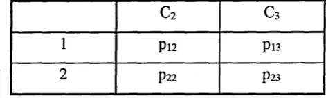
For an ordinal variable, a response variable Y, say, (note that the identification o f dependent and independent variables is unnecessary for odds ratios) with categories 1, ..., k, (k>2), in order to calculate an odds ratio one would have to collapse the data to binary in some way. If we consider first an original table with a binary explanatory covariate, X

:-Table 2.4: Probability distribution for a binary covariate and an ordinal response with k levels

Y=1 Y=2 * * * Y=k

X=1 P n P12 P lk

X=2 P21 P22 P 2k

Two possible ways o f collapsing this table to k-1 2x2 sub-tables are, firstly

:-Categorisation o f the response into all possible divisions o f ‘success’ and ‘failure’ or ‘favourable’ and ‘unfavourable’, assuming the categories are ordered ‘best’ (Y =l, say) to ‘worst’ (Y=k) in some sense, or similarly vice versa

:-Table 2.4.1: Category 1 vs Categories 2 to k

Y=1 Y=2 to k

X=1 _P11 P 1 2 + ... + P ik

X=2 P21 P 2 2 + ... +P 2k

Table 2.4.2: Categories 1 and 2 vs Categories 3 to k

Y=1 + Y=2 Y= 3 to k

X=1 P11+P12 P 1 3 + ... + P ik

Table 2.4.k-l: Categories 1 to k-1 vs Category k

Y=1 to k-1 Y= k

X=1 Pi i + ... + pik-i Pik

X=2 P21+ ... +P2k-1 P2k

When collapsing the data, it is important to consider the logic o f collapsing certain categories. For example, if you have a variable with categories ordered as very high, high, low and very low, combining the categories very high, high and low, or high, low and very low, can make interpretations o f the merged categoiy difficult, as the levels have contrary interpretations.

The odds ratios for the k-1 tables can be calculated, to give an idea o f the differences in effect on the different dichotomies o f the response. Sub-divisions in this manner form the basis o f logistic regression and proportional odds modelling procedures, for ordered categorical data with more than two categories. For the latter in particular, from this approach, insight may be gained into whether the odds ratios across the k-1 divisions are approximately constant or similar, with a view to using a global odds ratio to describe the odds o f ‘success’ vs ‘failure’ for the covariate.

Another way to collapse the response, assuming again that levels are ordered ‘best’ to ‘worst’ or vice versa, is to make the divisions according to membership o f the ‘most favourable’ category

available:-Table 2.5.1: Category 1 vs Categories 2 to k

Y=1 Y=2 to k

X=1 P n P12+ ... + P lk

X=2 P21 P22+ ... +p2k

Table 2.5.2: Category 2 vs Categories 3 to k

Y=2 Y= 3 to k

X=1 P l2 P 1 3 + ... + P ik

Table 2.5.k-1: Category k-1 vs Category k

Y=k-1 Y= k

X=1 Plk-l Pik

X=2 P2k-1 _{.... P2k_ .}

As mentioned for the previous collapsing o f the data, though only applying to the right hand side o f the dichotomy, it is important to make sure the collapsing o f categories does not make interpretation difficult, i.e. that no levels with contrasting meanings are combined.

The collapsing o f the response in this way allows comparison o f the odds that given an individual has responded in category j or worse, they have responded in the most favourable o f these categories available, j. The interpretations o f these odds ratios are different from those pertaining to ‘success’ and ‘failure’. Sub-dividing the response in this manner forms the basis for the continuation odds modelling procedure, which seeks to describe the k-1 tables above with a single global odds ratio.

2.2.6: M easures o f association for ordinal data

:-Table 2.6: Cross classification o f Own Morale bv Communication with More Senior Officers/Managers

Communication

Respondent’s Own Morale

Very High (VH)

High (H)

Neither

(N) Low(L)

Very Low (VL)

Very Good (VG) 51 142 71 33 7

Good (G) 58 302 244 120 37

Neither (N) 35 169 218 139 41

Bad (B) 5 54 65 103 38

Very Bad (VB) 1 5 14 13 27

Consider two individuals, one classified in the cell (VG, VH) and the other (G, H). This pair is concordant as the first subject is ranked higher than the second on both scales. Each o f the 51 subjects in cell (VG, VH) form concordant pairs when matched with each o f the 302 classified (G, H), so there are 51x302=15402 concordant pairs from those two cells. The 51 individuals classified (VG, VH) also form concordant pairs with each o f the other (244 + 120 + 37 + 169 + 218 + 139 + 41 + 54 + 65 + 103 + 38 + 5 + 1 4 + 1 3 + 27) individuals they are ranked higher than on both variables. Similarly, the 142 subjects in cell (VG, H) are part o f a concordant pair when matched with the (244 + 120 + 37 + 218 + 139 + 41 + 65 + 103 + 38 + 14 + 13 + 27)

individuals they are ranked higher than on both variables.

The total number o f concordant pairs, denoted by C, equals >

C = 51(302+244+120+37+169+218+139+41+54+65+103+38+5 +14+13+27)

+142(244+120+37+218+139+41+65+103+38+14+13+27) +71(120+37+139+41+103+38+13+27) +33(37+41+38+27) +58(169+218+139+41+54+65+103+38+5+14+13+27) +302(218+139+41+65+103+38+14+13+27)

+244( 139+41+103+38+13+27)

The number o f discordant pairs o f observations, D, is

:-D = 142(58+35+5+1) + 71(58+302+35+169+5+54+1+5) + ... + 103(1+5+14) +38(1+5+14+13)

= 334,075.

Therefore in this example, C>D suggests that lower morale has a tendency to occur with the feeling that communication is bad, and higher morale to occur with good communication.

A measure o f association that uses the above statistics is gamma, y, defined as the difference between the probabilities o f concordance and discordance (Goodman and Kruskal (1954)). For the sample case >

•/“^ ( C -D V C C + D).

As for a correlation coefficient, the range o f gamma is -1< y < 1, and as y -> |1|, the stronger the association between the two variables. Independence between variables implies that y=0, but the inverse is not necessarily true, as some non-linear association, eg a U-shaped joint distribution, may not be detected by gamma

:-Table 2.7: U-shaped joint distribution o f two variables X and Y

yi y2 ys

Xi 0.2 0 0.2

X2 0.2 0 0.2

X3 0 0.2 0

For the morale example above it was found that C = 736,012 and D =334,075. Of the concordant and discordant pairs, 68.78% are concordant and 31.22% discordant, therefore the difference in proportions gives y1131 = 0.376, indicating a moderately strong tendency for morale to be higher when communication with more senior managers/officers is deemed better. Measures o f association for ordinal variables are discussed fully in Agresti (1984).

2.3: Standard m odels m odified for ordinal variables

The following sub-sections briefly outline how some standard categorical modelling procedures can be adapted to accommodate ordinal information. The adaptation o f standard loglinear and logit models for ordinal variables hinges on the use o f scores for the levels o f explanatory variables, rather than the utilisation o f ordinality in a

dependent variable. These models are examples o f Generalised Linear Models (GLM). In brief, GLMs are a class o f models first developed by Nelder and Wedderbum (1972). GLMs are models basically specified by three components - A random component which identifies the probability distribution o f the response variable; a systematic component which specifies the form o f the model, in terms o f the linear function o f the explanatory variables; a link function which describes the relationship between the systematic component and the expected value (mean) o f the random component. Full details o f GLM’s are contained in McCullagh and Nelder (1989).

2.3.1: Scoring the levels o f ordinal variables

One o f the main objectives o f this research is to examine models and methods that do not require scoring o f the levels of an ordinal variable. However some o f the methods and examples described within this thesis require the assignment of scores, so that the ordinality o f a variable is utilised in some way, rather than lost to nominality.

the ‘distance’ between categories of an ordinal variable, and therefore assigning scores is often arbitrary.

Sometimes a score may be an actual numerical response, eg the number o f cancerous lungs (0, 1, 2), or the midpoint o f an interval, if the variable is a grouping o f an underlying continuous variable, eg age (<16, 16-25, 26-39, 40+) or salary (<£6k, £6k-£12k, £13k-£20k, £20k+).

Where no obvious choice o f scores exists, integer scores are often used. Assuming the levels o f an ordinal variable are equally spaced leads to easy interpretation o f statistics or models fitted for that variable (Koch et al (1977)).

Alternatively, if it is not appropriate to assume equal spacing, and there are suspicions or further information about inter-category distances, one could assign a variety o f ‘reasonable’ sets o f scores, to see if, or how much, substantive conclusions depend on the choice o f scores. One may settle for a set o f scores that gives the most desirable results, though care must be taken when interpreting and/or reporting results in such cases.

Another approach is to use distributional scores. In some cases it may be assumed that there is an underlying continuous measurement scale for which a particular

distribution, with distribution function F, is suitable, eg a normal or uniform

distribution. Scores for the categories of the variable could be functions o f the ranks. For example, scores may be estimated from the data by evaluating F_1(rj/(N+1)), where

Tj is the midrank score for category j, for j = l , ..., k, and N is the total number o f

observations. Many statisticians have voiced concerns over the use o f such scoring methods and prefer preassigned scores. For further discussion see Thomas and Kiwanga (1993).

likelihood estimation the package calibrates scores from a particular explanatory covariate, so that those scores are most likely to be associated with that covariate. A drawback to this method is that the scores vary with the choice o f calibration

instrument, i.e. explanatory variable, so substantive conclusions will therefore probably be dependent on the scores obtained.

Most methods o f assigning scores to the categories o f an ordinal variable and/or their interpretation are subjective. Methods o f estimating scores are dependent on the data used to calibrate them, and therefore not in accordance with a preconceived suspicion. Agresti (1984) gives some discussion on scoring. In this investigation preassigned integer scores and CHAID estimated scores are used, the motivation for which is to compare the results obtained by the different scoring methods.

2.3.2: Loglinear m odelling

Loglinear analysis models cell frequencies or probabilities from contingency tables, therefore there is no dependent variable as such. A loglinear model shows how the factors affect the distribution o f observations within the cells o f a table, and how the factors associate with each other.

Earlier, in section 2.2.2, it was seen that if two variables, X and Y, with levels i and j, are independent, then Tty = Tti+Tt+j for all i and j. Equivalently for expected cell

frequencies {mij=n7ty}, if X and Y are independent then mij=n7ii+7t+j for all i and j.

Therefore on a logarithmic scale, independence corresponds to

log my = log n + log Ki+ + log

7C+J-Referred to alternatively as

where jli is the overall mean o f the log cell frequencies, and the X parameters are the effects o f the variables X and Y, on the log cell frequencies adjusting for the overall mean.

This is called the loglinear model for independence. In standard loglinear modelling, the next more complex model is the saturated model (saturated means there are as many parameters in the model as cells) incorporating an interaction between the two variables

log niij = p. + X(X)i + ^(Y)j + ^(XY)ij (2.4)

Which is the most general model for two variables. It provides a perfect fit to the data and has no degrees o f freedom, i.e. it has a parameter for every cell, therefore it is not really useful, and shows nothing new.

However, if one or both o f the variables are ordinal, an unsaturated specialised loglinear model can be formed. Firstly suppose that X and Y are both ordinal with known category scores Uj and Vj respectively, then a simple model that utilises the ordinality in the variables and accounts for an association between them is

log my = [i + X{X)i + X{Y% + P(ui- u )(vj- v ) (2.5)

where u and v are the means o f the scores Ui and Vj.

This model is called the uniform association model. Note that this model only requires 1 more parameter than the independence model as opposed to ij extra parameters o f the saturated standard model, and does not require extra parameters if the number o f levels o f X and Y increases. This increase in efficiency is the biggest advantage o f such a model, further to the employment o f the ordinality in the variables (Haberman

association between X and Y, therefore if p=0 then the variables are independent. The

term P(ui- u )(vj- v ) reflects a deviation o f log m;j from the independence model. If p>0

then more observations are expected to have (large X, large Y) or (small X, small Y) values, than if X and Y were independent, and if p<0 one would expect more (large X,

small Y) or (small X, large Y) values.

If only one o f the variables, say Y, is ordinal with known category scores V j, a similar

model to that above is given by the row effects model

log my = |Ji + X(X)i + V )j + ^i(vj-v) (2.6)

The {Xi} are row effects (hence the name o f the model, although it can also be called the column effects model if it is the column variable that is ordinal). Within a particular row, i, the deviation o f log m;j from independence is a linear function o f the ordinal

variable. If T i= 0, X and Y are deemed to be independent. If T i> 0, then in row i the

probability o f classification above v on Y is higher than would be expected if X and Y

were independent. If T j<0 then observations in row i are more likely to be classified at

the lower end o f the scale o f Y.

These concepts in loglinear modelling can easily be applied to higher dimensions o f variables, for instance, consider another variable Z with k categories. If all 3 variables are nominal, a loglinear model more complex than the independence model but unsaturated, describing the association between the variables and the distribution o f observations would be

log m ij = JJ, + X(X)\ + ^(Y )j + ^(Z )k + ^(XY )ij + A,(XZ)ik + ^(Y Z )jk (2-7)

If all these variables are ordinal with X and Y having category scores Ui and Vj as for model (2.5) and Z with category scores Wk, a model utilising this information, equivalent to (2.7) but more parsimonious can be given by

:-log my = \i + XpQi + ^(Y)j + ?kz)k + P(xY)(ui-w )(vj-v ) + p(xz)(ui-« )(wk-n7)

+ P(yz)(vj- v )(w k- w ) (2 .8 )

which only has 3 more parameters than the independence model compared to (ij+ik+jk) more parameters than the independence model for (2.7).

If, say, X is nominal while Y and Z are ordinal, the row effects model (2.6) for 2 dimensions can be extended to give

log m jj = J I + X(X)i + ^(Y )j + ^(Z )k + X (X Y )i(V j-V ) + T(X Z)i(W k“

w

+ P(YZ)(vj-v )(wk-w ) (2.9)

where the X-Y and X-Z association terms have the same form as in the row effects model, and the Y-Z association term has the same form as in the uniform association model (2.5). This model, again, is more parsimonious than a model treating all variables as nominal.

The ordinality o f variables can be taken into account by these types o f models in different ways, also, for instance, log-multiplicative models are a form o f ordinal

loglinear models which estimate the scores Uj and Vj as parameters. For two ordinal

variables X and Y, if the ordered scores Ui and Vj from before are treated as unknown parameters m and Vj, the two dimensional log-multiplicative model is given by

which simplifies to the loglinear model for independence if p = 0. The score parameters

jii and Vj are estimated from the data to give the model best fit, and therefore probably should not be used for any other purpose than in the model itself.

2.3.3: Logit modelling

Logit models can be equated to loglinear models, but take a slightly different form, logit models describe the effects o f a set of explanatory variables on a response

variable, but do not describe associations between explanatory variables. Logit models with respect to ordinal explanatory variables are considered here, whilst in section 2.3.4, the binary logistic model is described in the context o f a basis for the more sophisticated proportional and continuation odds models.

Consider 3 categorical variables X, Y and Z with levels i, j and k respectively, where Z is a dichotomous response variable, {ftijk} and {m^} denote cell probabilities and frequencies. The conditional probability o f response k at levels i and j o f X and Y is 7tk(ij) = 7tijk/TCij+. The logit for Z is the log odds o f an event (a response)

log [ 7t2( ij/( l- 7 t2 ( ij) ) ]

= log (7Cij2/7Ciji)

= log (mp/mjji).

First suppose X and Y are nominal, the logit o f Z could be modelled by

log (niyVmiji) = a + i(X)\ + T(Y)j + 'fyxYjij (2.11)

Where a is the log odds that Z=2 in this case, if the % parameters are zero. {x(x)i}

pertains to the partial association between X and Z, and {T(Y)j} pertains to the partial

and Y on Z. If all T(x)r=0, then Z is conditionally independent of X, given Y, and the

same applies to Y and Z when all T(Y)j=0.

If X and Y are ordinal, with, as before, known category scores Ui and vj, in order to take into account this quantitative information, the logit of Z can be modelled by

log (mij2/miji) = a + p(X)(ui-w ) + P(Y)(vj-v) + P(XY)(ui-w )(vr v ) (2.12)

Where P(X) and p(y> represent local log odds ratios for the partial X - Z, and Y - Z

associations, and P(xy) represents the joint effects o f X and Y on Z therefore if P>0 the

log odds that Z=2, i.e. the logit of Z, increases. If all p parameters are zero, this means

that Z is independent o f X and Y.

If X is nominal and Y is ordinal with scores Vi, a combination o f the above logit models can be applied

log (mij2/miji) = a + x(X)i + P(Y)(yj- v ) + %Y)i(vj- v ) (2.13)

The interpretation o f parameters is the same as for the corresponding parameters in the two previous models (2.11) and (2.12).

Logit models (2.11), (2.12) and (2.13) can be fitted for higher dimensions o f variables similarly to loglinear models.

2.3.4: The Binary Logistic M odel

The binary logistic model is a fairly typical logit model, and in the description below does not account for ordinality in any o f the variables. The model is discussed in more detail, mainly because it is like a building block for the more sophisticated proportional and continuation odds models, which account for an ordinal response variable. The proportional and continuation odds models degenerate to the binary logistic model when the response variable has only two categories. Also when these more

sophisticated models fail to be appropriate, the binary logistic offers a method o f modelling the response in at least some context o f interest.

Let Y be a binary response variable where Y=1 for success and 0 for failure (possibly a dichotomised ordinal response). If there are m explanatory covariates, xi, x2, ..., xm, thought to influence success, then an individual, i, with specific covariates, x,-, has

probability o f success ft(x j). The response variable Y j follows a Bernoulli distribution.

The logistic regression model is given by

log {7c(x,) / [l-7C(x,)]} = Po + P'x,- (2.14)

where P' = (Pi, p2, ..., Pm), and x-, = (xu, x2i,..., xmi).

If we let rji = po + P'xi and rearrange the model formula above, the probability o f success can be obtained

7t(xi) = e x p ( r |i ) / [ l + e x p ( r i i ) ] ( 2 .1 5 )

The probability o f success, 7t(xj) is modelled via the logit transformation. This

transforms 7t(xj) from the range (0, 1) to the range (-«>, +oo)} so the parameters o f the

The binary logistic model is modelling the log odds of a successful response for an individual with specific covariates Xj. The p parameters show how changes in the values o f covariates affect the probability o f success.

To compare 2 individuals a and b, with covariates xa and Xb, the difference in log odds o f success is

log [7T(xa)/{ l-7T(xa)} ] - log [7t(xb)/{ l-7t(xb)} ] = P'(xa-xb)

rearranging

[rc(xa)/{ l-7 t(x a)} ]

log --- = P'(xa-xb) (2.16)

[7t(xb)/{l-7u (xb)} ]

Therefore P'(xa-xb) represents the log odds ratio o f success for an individual with covariates x a compared to an individual with covariates x b.

2.3.4.1: Parameter estimation for the binary logistic m odel

Consider a random sample o f N individuals, all with a set o f covariates, Xi, and a

response o f either success, Yj=l, with probability 7t(xj), or failure, Yi=0, with

probability l-Tt(xj). Yj is therefore a Bernoulli random variable, B {7t(xj)}, with

probability o f success related to po and p.

The likelihood is then proportional to a product of N such random variables

N

l « n7t(x,)Yi[i-7t(xi)]''Yi

i=l

Alternatively, Least Squares could be used to estimate the parameters. Iteratively reweighted least squares has similarities to Newton-Raphson. The statistical package SAS uses iteratively weighted least squares in the LOGISTIC procedure.

The methods o f estimation are asymptotically the same, and therefore converge to identical parameter estimates. However, often in the real world, with finite sample sizes, parameter estimates from the different estimation techniques will be very similar, but not exactly the same (Agresti (1984)).

2.3.5: Interactions between explanatory covariates

The following section briefly describes interaction terms, which are a little more complex to interpret than main effect parameters in any given model. If we have a categorical response variable Y (ordinal or binary) and two explanatory variables A and B, which could be o f any scale type, but for illustration’s sake, say, they are categorical, if the association between the response variable and A is the same within each level o f B (or vice versa), then there is said to be no interaction between A and B. In general, the absence o f interaction is characterised by a model which contains no second or higher order terms involving two or more variables.

If interaction is present, then the association between the response and A differs, or depends in some way on the level of B (or vice versa). The implication o f this is that any conclusions regarding the odds of a response for an individual with characteristic A should be made with respect to a specific level o f B, i.e. the effect o f A depends on the specific level o f B.

characteristic C should be estimated with respect to a specific level o f A and a specific level o f B.

Determining whether an interaction is present, i.e. significant, is fairly straightforward. One must first decide whether an interaction between two or more variables is plausible, and consequently if an interaction is logically possible, then a term is added to the model and its significance can be determined by a Wald Chi-square statistic, which measures the probability that the term is actually equal to zero, and therefore makes no significant improvement to the fit o f the model, as for main effects parameters (Wald (1943)).

The interaction parameter estimate on its own cannot be interpreted meaningfully, as the value o f an interaction term is an adjusting term, whereby the main effects o f two variables, say A and B again, at specific levels or values are combined and then adjusted by the value o f the respective interaction term to determine the effect o f a certain level A at a certain level of B. Discussion of interactions in logistic regression models can be found in Hosmer and Lemeshow (1989).

2.4: M odels for an ordinal dependent variable

2.4.1: The Ordinal Logistic Regression M odel

For an ordinal response variable, Y, with categories 1,..., K (K>2), ordinal logistic regression creates all possible dichotomies o f the variable, without violating the adjacency o f any pair o f levels. For example, if k=3, then dichotomies for calculating the odds o f category 1 versus 2 and 3, and categories 1 and 2 versus 3 are created, for given covariates. However, the odds of category 2 versus 1 and 3 are not estimated as the variable is assumed to fol