Abstract-Soft computing deals with imprecision, uncertainty, partial truth, and approximation to achieve practicability, robustness and low solution cost. As such it forms the basis of a considerable amount of machine learning techniques such as Artificial Neural Network, Support Vector Machines, Fuzzy Logic, Evolutionary algorithm and Swarm Intelligence. Oil and gas investment project is comprehensive and capital intensive engineering system characterized by uncertainty and high risk. The decision to invest is usually based on the evaluation of the project profitability which in most cases is not accomplished with high level of certainty. These economic evaluations are carried out with estimated set of parameters such as project costs, oil and gas prices, production profiles and inflation rate. The paper considers an approach to apply the concept of soft computing to uncertainty analysis in the economic analysis of oil and gas investment. A description of methods and models used for economic evaluation are provided. The application of soft computing such as support Vector Machines and Fuzzy Logic models are also provided. The soft computing approach is compared with basic evaluation without consideration for uncertainty. A case study is presented to illustrate that the data from which the evaluation is drawn are limited leading to an estimate that are inherently uncertain. The motivation of the proposed method is the fact that that the hybrid Support Vector Machines and Fuzzy Logic models have been used to predict oil prices, cost, net present value and internal rate of return with reasonable level of certainty. It also enables adequate risk assessment inherent in an investment to facilitate appropriate decision making.
Index Terms: Soft Computing, Industrial projects, Risk Assessment, Economic Evaluation, Uncertainty Analysis, Fuzzy Logic, Support Vector Machines, Profitability Indicators
I. INTRODUCTION
The decision to invest in the upstream oil and gas Industry based on the evaluation of the project profitability has been characterized by uncertainty and high risk. The focus of this paper will be on how to make people more aware of the risks and uncertainties in economic evaluations and to show the effects of these uncertainties on the economic indicators. Economic evaluations in the oil industry are carried out with cash flow models.Usually, these evaluations are carried out
with the estimated (most likely) set of parameters such as project costs, oil prices or reserves, are varied manually as to show their potential impact and sensitivities on profitability.In this paper, it is proposed to treat the uncertainties by using fuzzy Logic framework which was built on rule-based inputs from discipline experts. Prediction of oil prices, exchange rates, inflation rate and costs are accomplished using pattern recognition algorithm such as Support vector Machine(SVM). Some of the key uncertainties in oil and gas investments have been investigated in detail. To use soft computing technique for this purpose the following steps are required:
1. Build a discounted cash flow model of the project, 2. Identify the main uncertainties,
3. Develop model for the evaluations of these uncertainties The distribution of the profitability indicators will then show the estimated likelihood that the project will meet the required profitability criteria.Specific attention has been paid to the modeling of the following key uncertainties in typical oil and gas projects using Fuzzy Logic models: 1. The oil price,
2. The investment cost and operating expenses for the project,
3. The number of wells and associated capital cost to recover the reserves,
4. The oil and gas reserves and production profiles, 5. The inflation rate
II. BASIC CONCEPTS
A. Cash-Flow Concepts
Cash flow is the stream of monetary (Naira) values and consists of:
Cash inflow (revenue)-Product sales
Cash outflows(Cost)—resulting from a project development cost, cost of production(equipment purchases),cost of marketing, raw materials, components and labour.
The economic success occurs when cash inflow is greater than cash outflow. The measure of degree of this economic success can be expressed by various parameters including[1,4,6,8,9]:
Present Value
Pay-back period(discounted/undiscounted)
Internal Rate of Return
Profitability Index etc
B. Discounted Cash Flows and Project Profitability
When discounting, you simply want to know the worth of future amount now. In other words, it is to be examined if the same amount of money now is worth more than the
Applying Soft Computing Approach to
Uncertainty Analysis in Oil and Gas Economic
Evaluations
1
Odedele, T. O*, 2Ajoku K. B, 3Ibrahim H. D
.Correspondences
1,2Raw Materials Research & Development Council,(RMRDC)
Abuja Nigeria
1[email protected](Computer
Services Division)
2[email protected] Director Information and
Communication Department,(RMRDC) 3
same amount in the future. This is an aspect of the investment decision making where the interest rate plays an important role.Hence, by discounting, it is examined if it is worthwhile to invest a given sum of money at a particular interest rate. The decision to invest in a particular project is management decision after the accountant must have provided relevant information on the cost of investment alternatives and their expected returns. There are different ways by which such comparison between the cost of investment and expected returns can be made. In some instances, the discount rate which the project must maintain in order to yield expected return is given. The aim, here is to find the worth of the future cash flow now and examine whether or not the investment is worthwhile.This method is often called Present Value method. Investment with positive and higher present value is a better choice[14,15].
On the other hand, if the discount rate is not known, the aim in this case is to determine the interest rate at which the Present Value of the cash outflows equal to the present value of cash inflows. This interest rate is known as the internal Rate of Return. An investment is acceptable if the internal Rate of Return is greater than borrowing interest rate in the capital market and a project with higher internal Rate of Return is a better choice[14,15].The forecast of the annual amounts of money generated is called the cash flow of the venture. A company’s ability to add value is determined by its ability to generate future positive cash flows. Increasing value can be measured by Discounted Cash Flows (DCF). The DCF technique is used to determine the Net Present Value (NPV). The Net Present Value (NPV) is a function of the project results in dollars, the discount rate and the time period. The Net Present Value must therefore be quoted with the discount rate and the reference date. The reference date is the date to which future amounts have been valued. It is the date to which the Present Value is related. So the NPV is the sum over the years of the project of its discounted cash flow. This represents the value of the project to the investor.The profitability indicators result from “discounting” the cash flow. In this process the cash flow elements of later years are reduced by discount factors reflecting the time value of money. In the cash flow calculations of the oil field project different discount rates could be used; but discount rate of 22% is used in this paper. The model first calculates the gross revenue of a project from which royalties, costs and taxes should be subtracted. The gross revenues are simply the outcome of the production of oil (in barrels) and gas (in standard cubic feet) multiply by the oil and gas prices. After subtracting the royalties (not assumed in this case) the net revenuesremain. Before sharing of production, the contractor is allowed to recover costsout of revenues. Most PSCs will place a limit on cost recovery. In this case the cost recovery is limited to 40%. Revenues remaining after cost recovery are referred to as profit oil or profit gas, for which the contractor’s share of profit oil is assumed to be 40%. All the other elements like the (technical) costs, the future oil prices, the reserves, and inflation rate remain uncertain after contract signature. It is the petroleum economist’s job to advise on the economic attractiveness of the opportunities, taking into account the many uncertainties regarding reservoir behavior, development costs, future oil prices, and relationships with governments.The accuracy of the information used for generating the cash flow varies considerably. In order to
appreciate the effect of possible variations, a set of uncertainties will be defined, evaluated, and analyzed. Typical examples are changes in Oil prices, Oil reserves, Production behavior, Capital expenditure, Operating expenses and Time of production start-up.These uncertainties are contained in the project elements that are evaluated and analyzed. The four main elements are:
• Oil price • Costs
• Production Profiles • Inflation
III. OVERVIEW OF SUPPORT VECTOR MACHINES
Vapnik[18] proposed the support vector machines(SVMs) which was based on statistical learning theory. The governing principles of support vector machines is to map the original data x into a high dimension feature space through a non-linear mapping function and construct hyper plane in new space. The problem of regression can be represented as follows. Given a set of input-output pairs Z = {(x1, y1), (x2, y2), . . . ,(xℓ, yℓ)}, construct a regression function f that maps the input vectors x € X onto labels y € Y . The goal is to find a functionf ∈F which will correctly predict new samples. SVMs tackle the regression problem by finding the hyper-plane that realizes the maximum margin of separation between the classes. [18]. A representation of the hyper-plane solution used to predict a new sample xi is:
Y=f(x)=wi(x)+b (1)
where wi,(x) is the dot-product of the weight vector w and the input sample, and b is a bias value. The value of each element of w can be viewed as a measure of the relative importance of each of the sample attributes for the prediction of a sample. Various research studies have shown that the optimal hyperplane can be uniquely constructed through the solution of the following constrained quadratic optimization problem [16,18]
Minimise1/2||w||+C I (2a)
subject to _ yi(||w||+ b) ≥ 1 − i, i= 1, . . . , ℓ
i≥0,i=1,...,ℓ (2b)
In linearly separable problem, the solution minimizes the norm of the vector w which increases the flatness(or reduces the complexity) of the resulting model and hence the generalization ability is improved. With non-linearly separable hard-margin optimization, the goal is simply to find the minimum ||w|| such that the hyperplane f(x) successfully separates all ℓ samples of the training dataset. The slack variables i are introduced to allow for finding a hyperplane that misclassifies some of the samples (soft-margin optimisation) because many datasets are not linearly separable. The complexity constant C >0 determines the trade-off between the flatness and the amount by which misclassified samples are tolerated. A higher value of C means that more importance is attached to minimizing the slack variables than to minimizing||w||. Instead of solving this problem in its primal form of (2a) and (2b), it can be more easily solved in its dual formulation by introducing Langrangian multiplier α [11,16,18]:
In this solution, instead of finding w and b the goal now is find the vector α and bias value b, where each αi represents the relative importance of a training sample I in the classification of a new sample. To classify a new sample, the quantity f(x) is calculated as:
f(x)= sv αiyi i j
+b (4)
where b is chosen so that yif(x) = 1 for any I with C > αi>0. Then, a new sample xs is classed as negative if f(xs) is less than zero and positive if f(xs) is greater than or equal to zero. Samples xi for which the corresponding αi are non-zero are called as support vectors since they lie closest to the separating hyperplane. Samples that are not support vectors have no influence on the decision function.
Training an SVM entails solving the quadratic programming problem of (3a) and (3b). In SVMs, kernel functions are used to map the training data into a higher dimensional feature space via some mapping φ(x) and construct a separating hyperplane with maximum margin. This yields a non-linear decision boundary in the original input space. Typical types of kernels are:
− Linear Kernel: K(x, z) =
− Polynomial Kernel: K(x, z) = ( )d − RBF Kernel: K(x, z) = exp(−||x−z||2
/2σ2 ) − Sigmoid Kernel: K(x, z) = tanh(γ* − θ)
This condition ensures that the solution of (3a) and (3b) produces a global optimum. The functions that satisfy Mercer’s conditions can be as kernel functions.As promising as SVM is compared with ANN as regards generalization performance on unseen data, the major disadvantage is its black box nature. The knowledge learnt by SVM is represented as a set numerical parameters value making it difficult to understand what SVM is actually computing.
IV. METHODOLOGY
The system is divided into three parts: as it makes use of different systems for uncertainty analysis in the economic evaluation of oil and gas projects.
a. Prediction of oil prices, costs, inflation rates using Fuzzy Support Vector Machines (FuzzySVM). b. Prediction of production profiles using reservoir
engineering techniques
c. Uncertainty analysis in the economic evaluation of oil and gas projects using fuzzy logic approach.
A. Oil Prices
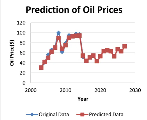
The history of oil prices has seen big fluctuations starting from the year 1986. The reason for the decrease in the 1980s was due global economic recession arising oil glut in the market. The price however pick up between 2005 and 2013. The downward trend began to shown in 2015. Historic fluctuations of the oil prices can be used as basis to predict future fluctuations. Fluctuations of oil prices will have effects on the economical results of any oil and gas project which a company intends to implements in the future because the e pected project’s earnings depend very strongly on the oil prices. The observed history and the predicted oil prices( in Fig1) shows that there is the real need to be careful with the economic calculations and to take into consideration the different ways the future oil prices may fluctuate. Through analysis of the history and forecast of the oil prices the inherent risks and uncertainties
in several scenarios may be identified. Fuzzy Support Vector Machines approach was applied to predict the future behavior of crude oil prices.The predicted oil prices for the ten years are as shown in Fig 1.
B. Costs
Project costs represent how much is going to be spent during the construction and the implementation phase of the project. The project results depend very strongly on the magnitude of the costs. If the costs are higher than estimated, the project’s profit will be less than expected. In some cases higher costs can lead to a big loss, especially when the profit is low or in case the project’s revenue is very dependent on the amount of the costs.
C. Production Profiles and Reserves
[image:3.595.306.563.363.573.2]The forecasting of production profiles is an iterative process, in which information gained from appraisal wells and actual production is continuously used by the reservoir engineers to update their previous views. The confidence level of the forecast will therefore be fairly low in the early stage of the venture and will be higher after the field has been producing for a few years. Key factors influencing the production profile include the amount of oil (or gas) in place, the drive mechanism, the fluid properties, and the initial rate of wells.
Fig 1 Prediction of Oil Prices
D. Inflation Rate
Inflation is a general rise in prices across the economy. This is distinct from a rise in the price of a particular good or service. Individual prices can rise and fall all the time in a market economy, due to consumer demand. Inflation occurs when most prices rise by some degree across the whole economy.
V. CASE STUDY
A. Field Development History
The sandstone reservoir was discovered by A1 well in Oct. 2003. Three additional delineation wells were drilled to help
0 20 40 60 80 100 120
2000 2010 2020 2030
Oil
Price($)
Year
Prediction of Oil Prices
define the extent of the field. A2 along the west flank while AN and AH at the northern and Eastern extremities of the structure respectively. Development drilling began from one centrally located platform in 2003. By Jan. 2010 a total of 13 wells (12producers and 1 observation) had been drilled. The completion of the development wells was with 7- in casing, 2 7/8- in tubing set on a packer through 7400ft. Most of the wells flow naturally as from 2005.
B. Geology
The formation in this field comprises of a homogeneous sandstone unit. The available geological information indicates that there was no water encroachment and gas cap. The planimetery of each contour yields the area as 4.86 acre. The contour interval, h = 246ft
C. Rock and Fluid Characteristics
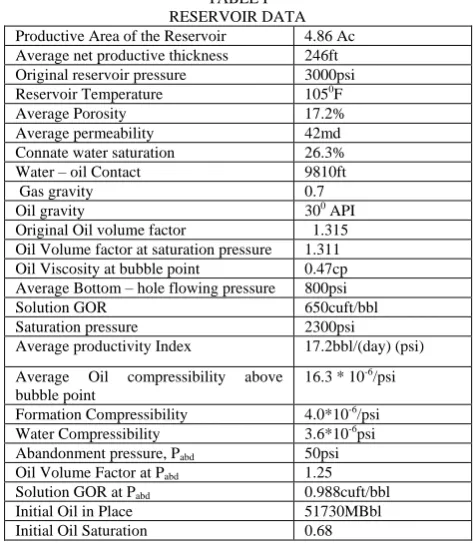
[image:4.595.301.556.145.237.2]Log Analysis data were available for nine wells. The data were used to evaluate porosity and water saturation. The log run was the conventional electric logs. The average core porosity, mean permeability and initial water saturation are as shown in Table I
TABLE I RESERVOIR DATA Productive Area of the Reservoir 4.86 Ac Average net productive thickness 246ft Original reservoir pressure 3000psi
Reservoir Temperature 1050F
Average Porosity 17.2%
Average permeability 42md
Connate water saturation 26.3%
Water – oil Contact 9810ft
Gas gravity 0.7
Oil gravity 300 API
Original Oil volume factor 1.315 Oil Volume factor at saturation pressure 1.311 Oil Viscosity at bubble point 0.47cp Average Bottom – hole flowing pressure 800psi
Solution GOR 650cuft/bbl
Saturation pressure 2300psi
Average productivity Index 17.2bbl/(day) (psi)
Average Oil compressibility above bubble point
16.3 * 10-6/psi
Formation Compressibility 4.0*10-6/psi
Water Compressibility 3.6*10-6psi Abandonment pressure, Pabd 50psi
Oil Volume Factor at Pabd 1.25
Solution GOR at Pabd 0.988cuft/bbl
Initial Oil in Place 51730MBbl
Initial Oil Saturation 0.68
[image:4.595.49.286.336.608.2]The relative permeability data are as shown in Table II
TABLE II
GAS AND OIL RELATIVE PERMEABILITY DATA Total Saturation (Sw+So) % Kg/Ko
0.20 0.0
0.40 5.5
0.60 0.55
0.70 0.170
0.80 0.555
0.90 0.0
D. Reservoir performance History
The Reservoir performance history of this reservoir is given in Table III. The primary production phase began in March 2005 and oil production reach about 33,000B/D from eight well in April 2006. The oil rate declined steadily at a rate of 25% per year.
TABLE III
RESERVOIR PERFORMANCE HISTORY Year Pressure
psia
Production rate B/D
GOR cuft/bbl
Watercut
2005 3000.00 0.0 650.0 0.0
2006 2800.00 33000.0 650.0 0.0
2007 2590.00 30751.0 650.0 0.0
2008 2450.00 28655.50 650.0 0.0
2009 2360.00 26702.69 650.0 0.0
2010 2250.00 24882.96 650.0 0.0
In the year 2010, a pressure maintenance program was proposed in order to arrest further reservoir pressure decline.Two exploitation alternatives to be examined are as follows:
Base Case F1 is the continuation of the existing exploitation plan using current depletion drive mechanism
[image:4.595.299.556.456.758.2]Case F2 is the crestal gas injection as of October 1, 2011. It is assumed that three quarter of the produced gas is to be injected into the reservoir. In the case of gas injection, it was assumed that the injected gas had the characteristic as the solution gas. The original reservoir fluid was greatly under-saturated. There was no water encroachment and water production. It is therefore required to predict the oil production in the next 25years in each case given the PVT, Viscosity and relative permeability data of the field as shown in Table IV:
TABLE IV
PVT AND VISCOSITY RATIO Pressure
psia
Oil Volume Factor,Bobbl/STB
Solution GOR, Rs
SCF/STB Gas Deviation Factor, Zat 1090F
Viscosity Ratio
Uo/Ug
3000 1.315 650 0.745 53.91
2500 1.325 650 0.680 56.60
2300 1.311 618 0.663 61.46
2100 1.296 586 0.652 67.35
1900 1.281 553 0.651 74.33
1700 1.266 520 0.660 81.96
1500 1.250 486 0.685 91.56
1300 1.233 450 0.717 102.61
1100 1.215 412 0.751 115.20
900 1.195 369 0.791 129.96
700 1.172 320 0.832 148.89
500 1.143 264 0.878 170.83
300 1.108 194 0.925 196.78
100 1.105 94 0.974 219.89
[image:4.595.297.555.460.758.2]Calculate oil production profile. The exploitation plan is depletion Drive mechanism. The initial oil in place was estimated as 51.73MM STB by volumetric method.
Several cost components and assumptions that were taken into account for economical calculation are briefly explained below:
The royalty rates currently range from a minimum of 12.5 percent to 18 percent with the average rate of 17% per gross revenue that is currently being offered.
Lease acquisition payments can range from several hundred dollars per acre to over $2,000,000.00 per acre.
Site Preparation and Permission fees -For a total wellbore length of about 10,000 feet, an application fee of $520,000.00 and a bond amount of $500,000.00 is required. The approximate costs associated with prepping a site for drilling amount to roughly $15,000,000.00.
Petroleum income tax rate of 85% was utilized to the analysis.It is assumed that the offshore field will be developed by use of jack-up drilling platform. Hence, the drilling and completion costs associated with a 8000 ft long about $140,000,000.00. However, the yearly operating and maintenance cost had been estimated to be $36,210,000.00. The utilities, direct and indirect labour, contingencies and preproduction expenses are $10,320,000.00,
$12,500,000.00, $9.000,000.00, $26,320,000.00 and
$15,000,000.00 respectively
For CaseF2 (Crestal gas injection), the utilities, direct and indirect labour, contingencies and preproduction expenses
are $25,320,000.00, $12,500,000.00, $9.000,000.00,
$60,000,000.00 and $30,000,000.00 respectively.
Additional drilling cost is $110,000,000.00 and yearly operating cost is $70,210,000.00. Other financial assumptions N204.00=$1.00 as at October 2015
(i). Capital cost for each project is to be financed by Bank loan. This loan is to be amortized over 5years at an interest rate of 32 percent.
(ii). Price of crude oil is to predicted using Fuzzy Support Vector Machines(FuzzySVM)
(iii). Discount rate is assumed to be 22%.
(iv). Overall inflation rate is assumed to be 10% per year. (v). Property production taxes are assumed to 4.6% plus vat rate of $0.0025 per bbl.
(vi). Tangible cost were depreciated using a straight line depreciation method
Appraise the exploitation scheme on a 25years horizon, and compute the measure of project worth, that is, net present value, Profitability Index, internal rate of return, benefit-cost ratio and investment – benefit ratio.Under the current circumstances, which scheme(CaseF1 or CaseF2)will you recommend for the development of this field to your management for consideration and approval?
VI. RESULTS OF ECONOMIC ANALYSIS
Economic analysis was performed based on 25 years of forecasted oil production for the field. The oil prices was predicted using Fuzzy Support Vector Machines(FSVM) as shown in Fig 1. The cash flow statement was constructed based on above-mentioned assumptions and the net present value and internal rate of return, payback period and profitability Index were calculated in order to determine the
overall profitability of the wells. Table V shows a summary of results of the field under the 25-year production.
TABLE V
RESULTS OF ECONOMIC ANALYSIS
Oil Produ ction
Cum. Oil Productio n(STB)
Total Income after Tax ($)
Net Present Value ($)109
IRR %
Pay Back period (years )
Produ ctivity Index
Case F I
6836298.0 369750592.0 3.7836 27.1 8.45 19.7
Case F2
8301640.0 425620416.0 1.1289 76.6 1.05 5.89
Case I-Depletion Drive, Case II-Depletion Drive with Gas injection after 6 years of production
Based on the positive NPV and acceptable IRR(>discount rate), the oil production under the assumption and values used in this analysis was found to be profitable based on 25-yeare production in both cases. But, unfortunately the assessment of uncertainty/risk has not been addressed. In the next section, the analysis will be the main focus using fuzzy logic inference model.
VII. UNCERTAINTY ANALYSIS USING FUZZY LOGIC APPROACH
Fuzzy Logic which was introduced by Lotfi A. Zadeh was based on fuzzy sets in 1965 [20,21,22]. The basic concept of fuzzy logic is to consider the intermediate values between [0,1] as degrees of truth in addition to the values 1 and 0. The following sections will briefly discuss the general principles of fuzzy logic, membership functions, linguistic variables, fuzzy IF-THEN rules, combining fuzzy sets and fuzzy inference systems (FISs).
A fuzzy inference system (FIS) is made up of five functional components. The functions of the five components are as follows:
1. A fuzzification is an interface which maps the crisp inputs into degrees of compatibility with linguistic variables. 2. A rule base is an interface containing a number of fuzzy if-then rules.
3. A database defines the membership functions (MFs) of the fuzzy sets used in the fuzzy rules.
4. A decision-making component which performs the inference operation on the rules.
5. A defuzzification interface which transforms the fuzzy results of the inference into a crisp output.
Notice that “if – then” rules may be used to both model the state of a system and to take a decision to control the system[7,10,12,13,17].
R1: If Profitability Index is High and Internal rate of return is High and Payback period is Low then there is no economic viability risk. Take as example the following set of “if – then” rules constituting a fu y control-model for economic viability risk assessment system:
R2: If Profitability Index is High and Internal rate of return is Low and Payback period is Low then there is no economic viability risk.
The economic viability risk assessment is carried out by analy ing the fu y rules derived from e pert’s knowledge and experimental data. The fuzzy model is constructed with three inputs and single output (TISO). The Profitability Index, payback period andInternal rate of return are considered as inputs and economic viability Risk is chosen as output for the fuzzy model. The input variables are classified into three membership functions such as low, Normal and high. The output variable is classified into three membership functions such as No risk, Low risk and high risk.
TABLE VI
MEMBERSHIP FUNCTIONS FOR INPUT VARIABLES
TABLE VII
MEMBERSHIP FUNCTIONS FOR OUTPUT VARIABLES
The relationship between input and output variables is established through fuzzy rules as shown in table VIII. Linguistic rules describing the fuzzy system consists of 27 rules(33). It may not be necessary to evaluate every possible input combination, since some may rarely or never occur.
TABLE VIII FUZZY RULES
L: Low; N: Normal; H: High: NR:NoRisk: LR:Low Risk:HR:High Risk RPI:RelativeProfitability Index
[image:6.595.306.552.49.158.2]Through the experience of the operator, few rules can be evaluated thus simplifying the processing logic.The trapezoidal shape of each Linguistic variable are as shown below:
Fig 2 Profitability Index
[image:6.595.305.550.195.432.2]Fig 3 Internal Rate of Return(IRR)
Fig 4 PayBack Period
Fig 5 Economic Viability Index
VIII. RESULTS AND DISCUSSION
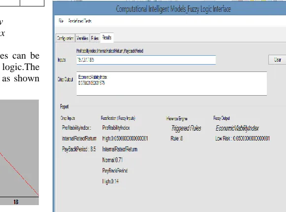
The simulation study is carried out by computer program called Fuzzinator(Fuzzy Logic Controller) for following cases:
CaseFI (Depletion Drive Mechanism): Profitability Index: 19.7, IRR: 27.1, Payback period:8.5.
Fig 6 Economic Viability risk assessment Results for CaseI
Low Normal High
Profitability Index
0- 4.9 4.7-12.8 12.5-20.0
Internal rate of return(%)
0-DiscountRate
(DiscountRate-2)- 55.0
50.0- 200.0 PayBack
Period(Years)
1-5 4-6 5-50
No Risk Low Risk High Risk
Economic viability Index
0.4-1.0 0.2-0.5 0-0.3
Rules 1 2 3 4 5 6 7 8 9
Internal rate of return
H L N N N N H L H
Profitabili ty Index
H H H N L H N L L
PayBack Period
L L L N N N H H H
RPI N
R
NR N
R
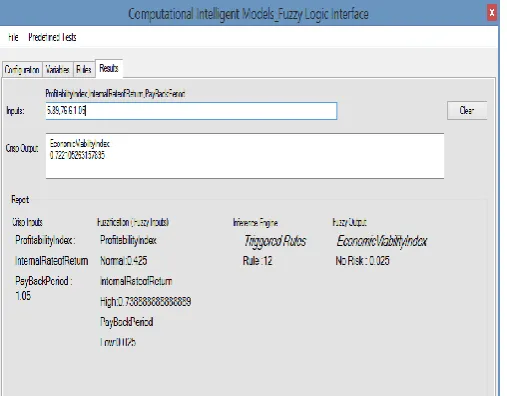
[image:6.595.41.293.433.565.2] [image:6.595.249.540.556.771.2]CaseF2(Depletion Drive Mechanism with crestal gas injection): Profitability Index: 5.8, IRR: 76.6, Payback period:1.05.The results obtained through computer simulation with three membership functions of trapezoidal shapes as shown in Figures 6 &7.
[image:7.595.40.294.190.388.2]Even though both cases are found to be profitable based on the positive NPV and acceptable IRR(>discount rate), CaseFI however has inherent low investment risk(Fig 6) while CaseF2 has no risk(Fig 7).
Fig 7 Economic Viability risk assessment Results for CaseII
IX. CONCLUSION
This study develops a novel model fuzzy logic system to characterize and assess the risk and uncertainty associated with economic evaluation of oil and gas upstream projects. The study and understanding of the fuzzy Logic technique and its role in uncertainty analysis tasks are done. This technique is then implemented in the Microsoft C# programming language to perform uncertainty analysis task for the economic evaluation of oil and gas upstream projects. This approach is rather more significant than the conventional economic analysis used for oil and gas projects because it is important to assess the risk associated with the investment even if the project is viable judging from the economic indicators. In view of the above discussion, CaseF2 (Depletion Drive with gas injection after 6 years of production) should be implemented because the project has no economic viability risk compared with CaseFI(Depletion Drive without gas injection) which has low economic viability risk despite the fact that the profitability criteria are favorable.
REFERENCES
[1] Barish, Norman N: Economic analysis for Engineering and Management Decision Making 2ndedMcGraw Hill Book Company
New York 1978.
[2] J. L. Castro and M. Delgado, “Fu y systems with defu ification are universal appro imators,” IEEE Transactions on System, Man and Cybernetics, vol. 2
[3] Chen Y, Wang J: Support vector learning for fuzzy rule-basedclassification systems. IEEE Transactions on Fuzzy Systems 2003,11(6):716-728.
[4] Clifton D. S. (Jnr) and D. E Fyffe: Project Feasibility Analysis: A guide to Profitable Ventures.
[5] Cristianini N, Shawe-Taylor J: An Introduction to Support Vector Machines and Other Kernel-Based Learning Methods Cambridge, U.K.: Cambridge UniversityPress; 2000.
[6] Deborah S. Kezsbom, Donald L. S and Katherine A. E: Dynamic Project Management: A Practical guide for Managers and Engineers. [7] Dubois D, Prade H: Operations on fuzzy numbers. International
Journal of Systems Science 1978, 9(6):613-626.
[8] E.A Frohlich,P.MHawranek, C.F Lettmoyr,J H. Pichler, “Manual for Small Industrial Businesses -Project Design and Appraisal.1994 UNIDO
[9] Ferguson C. E and Maurice S. C. Economic Analysis Home Wood III Richard D. Irain 1970..
[10] K. Tanaka, An Introduction to Fuzzy Logic for Practical Applications. N.Y.: Springer, 1997.
[11] Lin CF, Wang SD: Fuzzy support vector machine. IEEE Transactions onNeural Networks 2002, 13(2):464-471.
[12] L.P. Holmblad and J.-J. Østergaad , “Control of a cement kiln by fu y logic,” in Fuzzy Information and Decision Processes,M.M. Gupta and E. S´anchez, Eds. Amsterdam: North Holland, 1982. [13] M. K. Mishra, S.G. Tarnekar, D. P. Kothari, Arindam Ghosh
“Detection of incipient faults in single phase Induction motors using Fu y logic; “Proceedings of IEEE International Conference on Power Electronics, Drives and Energy systems for Industrial Growth, New Delhi, January 1996”, pp. 117-121.
[14] Omuya J. O. Business Accounting Volumes 1 & 2 1985
[15] Odedele T O ,Jolaoso M A, FolarinOkuribido& A P Onwualu: “Computer Aided Project Appraisal- Kagara Talc Processing Plant As A Case Study” 2010
[16]Sch¨olkopf, A. Smola, R. C. Williamson, and P. L. Bartlett “New support vector algorithms”. Neural Computation, 12:1207–1245 2000.
[17] Takagi T, Sugeno M: Fuzzy identification of systems and its applicationsto modeling and control. IEEE Transactions on Systems, Man, andCybernetics 1985, 15:116-132.
[18] V. Cherkassky and Y. Ma “Practical selection of SVM parameters and noise estimation for SVM regression,” Neural Networks, vol. 17, pp. 113–126 2004.
[19] Z. Y. Luo, P. Wang, Y. G. Li, W. F. Zhang, W. Tang and M. Xiang, “Quantum-inspired evolutionary tuning of SVM parameters,”
Progress in Natural Science, vol. 18, pp. 475–480, 2008.
[20] Zadeh, L. A., 1965. Fuzzy sets. Information and Control, vol, 8, pp, 338–353.
[21] Zadeh, L. A., 1973. Outline of a new approach to analysis of complex systems and decision processes. IEEE Transactions on Systems, Man, and Cybernetics, vol. 3, pp. 28–44.
[22] . ZadehL.A, “The concept of a linguistic variable and its application to appro imate reasoning,” Information Sciences, no. 8, pp. 199–249, 301–357, 1975.
Dr Ibrahim Doko Hussaini who hails from Doko Niger state of Nigeria was born on 23rdSeptember 1962. The educational background is as follows: * TheUniversity of Leeds, United Kingdom(1993 )Ph.D(Textile Science & Engineering), He is currently Director General of Raw Materials Research & Development Council,(RMRDC) Abuja Nigeria
Engr Timothy.O Odedele who hails from Ipetumodu, Osun state of Nigeria was born on 29th April 1958. The educational background is as follows: * B.Sc. Petroleum Engineering (Second class Upper Division1984) University of Ibadan, Ibadan * Post Graduate Diploma Computer Science from Federal University of Technology, Minna,* M.Sc Computer Science -Universityof Ibadan, Ibadan .He works with Raw Materials Research & Development Council, Abuja Nigeria. He is currently Deputy Director(Computer Services Division)