Study of the LiDAR accuracy in mapping forest road alignments and estimating the earthwork volume

JOURNAL OF FOREST SCIENCE, 64, 2018 (11): 469–477 https://doi.org/10.17221/87/2018-JFS

Study of the LiDAR accuracy in mapping forest road

alignments and estimating the earthwork volume

Benyamin MATINNIA*, Aidin PARSAKHOO, Jahangir MOHAMADI,

Shaban SHATAEE JOUIBARY

Department of Forestry, Faculty of Forest Science, Gorgan University of Agricultural Sciences and Natural Resources, Gorgan, Iran

*Corresponding author: [email protected]

Abstract

Matinnia B., Parsakhoo A., Mohamadi J., Shataee Jouibary S. (2018): Study of the LiDAR accuracy in mapping forest road alignments and estimating the earthwork volume. J. For. Sci., 64: 469–477.

Today, differential geographical position system and total station devices are improving the accuracy of positioning information, but in critical locations such as steep slopes and closed canopy cover, the device accuracy is limited. Moreover, field surveying in this technique is time-consuming and expensive. For this reason, remote sensing technique such as light detection and ranging (LiDAR) laser scanner should be used in field measurements. The objective of this study was to evaluate and compare precision and time expenditure of total station and airborne LiDAR in producing horizontal and vertical alignments and estimating earthwork volume of two proposed forest roads in a deciduous forest of Iran. To investigate this task, the geographical position of proposed forest roads were detected by differential geo-graphical position system and then marked on land. Mentioned roads were taken again with Leica Total Station (LTS) on control points with same 5 m intervals from start point. Recent data served as a reference value for comparison with LiDAR measurements. The data were processed in Civil 3D, Fusion and Leica geo office software. Results showed that in comparison to field-surveyed routes by LTS, the LiDAR-derived routes exhibited a horizontal accuracy of 0.23 and 0.47 m and vertical accuracy of 0.31 and 0.66 m for road 1 and road 2, respectively. The LiDAR-derived sections every 1 m exhibited cut and fill accuracy of 2.39 and 3.18 m3 _{for road 1 and 2.98 and 5.60 m}3 _{road 2, respectively. In} this study, it was proved that the road project can be prepared faster by LiDAR than that of LTS. Therefore, high ac-curacy of road projection by LiDAR is useful for terrain analysis without the need for field reconnaissance.

Keywords: airborne LiDAR; Leica Total Station; mapping proposed road; accuracy estimation; deciduous forest canopy cover

Updated terrain information generated from light detection and ranging (LiDAR) can serve for-estry purposes especially road projection under the closed forest canopy cover (Mena, Malpica 2005; Akay 2006; Amo et al. 2006). Forest road projection is conducted along with field survey (Clode et al. 2007; Coffin 2007). Field survey of horizontal and vertical alignments of roads is ex-pensive and time-consuming and sometimes have low accuracy especial in large-scale surveying. The cost-effective method in analysis large-scale objects is remote sensing techniques which the

oldest is aerial photo interpretation (Alharthy, Bethel 2004; Espinoza, Owens 2007). Providing elevation data and digital elevation model is the most important stage of terrain mapping by re-mote sensing techniques. Digital elevation model has more accuracy if the density of elevation data to be high (Umeda et al. 2007; David et al. 2009; Grote et al. 2012).

(Krogstad, Schiess 2004). LiDAR aerial laser scanner is used to collect three dimensional (3D) data (Hickerson 1964; Ferraz et al. 2016). De-tection and vectorisation of urban, rural and for-est road network are one of the jobs of LiDAR. LiDAR technology is similar to radar and some-times is called laser radar. The difference between these two technologies is that radar applies radial wavelength whereas LiDAR applies aerial infrared laser. The prevalent technique in determining the distance to an object or surface is the transmis-sion of the laser pulse. With the use of the LiDAR, the information can be collected under a difficult condition such as low light angle, cloudy weather, dense canopy cover and darkness (Liu, Sessions 1993; Hinz, Baumgartner 2003).

Not only the horizontal alignment but also lon-gitudinal section and position of the project line are effective in selecting the best route (Coulter et al. 2001). In some projects, various models have been used to optimise project line and decrease the cost of road planning and construction, but most of these models could not do accurate due to the lack of accurate elevation data about longitudinal section (Evans et al. 2009; Chekole 2014). High-resolution digital terrain model extracted from LiDAR can be used to produce rapid, easy and ac-curate longitudinal section of road. 80% of the total investment of forest road construction project on steep slopes is assigned to earthwork (Umeda et al. 2007). Therefore, an accurate estimation of earth-work volume is necessary for the improvement of monitoring projects and cost control. Surveying cross sections of road are conducted to calculate earthwork volume of proposed roads (Ichihara et al. 1996; Lacoste et al. 2005). Accurate cross sections of hillside can be provided by elevation data of aerial LiDAR technology in short distances (less than 20 m) and under the closed forest cano-py cover. The LiDAR technology is used to obtain the terrain elevation data. Airborne and terrestrial LiDAR sensors are used for scanning the earth surface. The resulting data is stored in files called point clouds (Hui et al. 2016; He et al. 2017).

In recent years accurate digital terrain model has provided interesting consequence in recording and analysis of elevation data and thus engineers could evaluate large volume data about geometric plans of linear objects such as roads in an extensive area in short time. Therefore, this basic information tech-nology could reduce the volume of time-consum-ing field works in forest road planntime-consum-ing and mapptime-consum-ing project. The purposes of this research were: (i) to prepare the horizontal and vertical alignments of

road alternatives from LiDAR data, (ii) to estimate the earthwork volume for the proposed forest roads using digital terrain model of LiDAR and compare the accuracy of this technique with field surveying by Leica Total Station (LTS) device (TS10; Leica, Switzerland).

MATERIAL AND METHODS

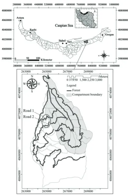
Study area. District two in Dr. Bahramnia forest with an area of 1,992 ha is located from 36°42'30''N to 36°43'30''N and 54°21'6''E to 54°23'30''E in Go-lestan province and watershed No. 85. The total length of proposed forest roads in this district is 28 km (21 km is located in timber compartments with an area of 995 ha). The forest is mixed

decidu-ous dominated by trees species of Parrotia persica

(de Candolle) C.A. von Meyer, Carpinus betulus

Linnaeus, Fagus orientalis Lipsky, Quercus casta-neifolia C.A. von Meyer and Zelkova carpinifolia

(von Pallas) C. Koch. The mean of trees density per hectare was 214.92 and the canopy cover was 75 to 85%. First proposed road (road 1) with a length of 365 m and the second proposed road (road 2) with a length of 495 m were selected in this study (Fig. 1).

Ground-based surveying by LTS. Leica Total Station was used in field surveying and Leica Geo Office software (Version 8.3, 2014) was used for data processing. The total station is a surveying de-vice that combines the angle measuring capabilities of theodolite with an electronic distance measure-ment to determine the horizontal angle, vertical angle and slope distance to the particular point. The collimation of the device was done for levelling and then the coordinate of the device was recorded by differential geographical position system as the ref-erence point. A start point (No. 0) on the road was determined and then measuring points at the same 5 m intervals from that point was set out (White et al. 2010). Indeed 73 and 100 control points were taken by LTS on road 1 and road 2, respectively. The direct distance and angles between a target staff on point No. 0 and a device was recorded and at the next stage coordinates (x, y, and z or north-ing, easting and elevation) of surveyed points rela-tive to the total station position. The device uses a beam of infra-red light to measure the distance. The velocity of this light in the atmosphere varies according to the temperature and pressure (Vene-ziano et al. 2002). Temperature and pressure were taken at the midpoint of the line. All cross sections were extracted every 10 m from each side of the centre line and perpendicular to it (3 points). The cross section survey sub-menu allows for measure-ments of earthwork areas which can be uploaded into AutoCAD Civil 3D (Version 2012) for earth-work volume calculations. The corrected horizon-tal distances (H) and height differences (V) were calculated using Eqs. 1 and 2 (Souleyrette et al. 2003; Türetken et al. 2013):

2

1 2

sin sin cos

K

H S Z S Z Z

R



      (1)

where:

S – slope distance after atmospheric correction, Z – vertical angle,

K – atmospheric refraction constant (0.142), R – radius of the earth (6.372 × 106_).

2 2

1

cos sin

2 K

V S Z S Z

R



     (2)

The analysis was repeated three times to evaluate the precision of the measurement.

Processing LiDAR data. LiDAR data were tak-en by RIEGL LMS-Q5600 laser scanning system (RIEGL Laser Measurement Systems GmbH, Aus-tria) mounted to an aircraft planned by the Rayan Naghsheh Company in October 2011 in leave-on tree condition. The average density of the points

on the surface was 4 points per m2_{. More}

informa-tion about LiDAR has been illustrated in Table 1. Preprocessing was done on original LiDAR data to remove random errors and then produced an ac-curate and high-resolution digital elevation model (DEM) from first and second ground pulses with Kraus and Pfeiffer algorithm with a spatial reso-lution of one meter. This step was done in Fusion software (Version 360_2, 2015). At the next step, the cloud points of a small part of DEM around the selected road were recalled in AutoCAD Civil 3D (Version 2014) and then the cloud points were converted to surface. A point cloud is a collection of 3D data that represents ground, vegetation, wa-ter, and other natural and man-made objects. Point cloud data is commonly stored in binary LAS (.las),

text ASCII XYZ (.xyz), and in a number of other

file formats. The vertical alignment, cross section and horizontal alignment were created from a sur-face layer with a resolution one meter. The analysis was repeated three times to evaluate the precision of the measurement (Sessions et al. 2010; Sidle, Ziegler 2012).

Mapping in AutoCAD Civil 3D. Horizontal alignment was created using the Alignment Layout Tools in AutoDesk AutoCAD Civil 3D. Freehand drawing tools for lines, curves and spirals were ap-plied based on azimuth and distances. Free curve fillet was designed between two entities by select-ing radius. Vertical alignment was created from an external file that contains a series of stations along an alignment, the elevation of each station, and op-tionally, the length of the curve at the station. Pro-file Layout Tool was used to add the project line and to analyse vertical tangents and curves. The profile elevation differences report (project num-ber) displays the station, existing ground elevation, design elevation and the elevation differences on

´

´

´

´

Table 1. Some characteristics of RIEGL LMS-Q5600 laser scanning system (RIEGL Laser Measurement Systems GmbH, Austria)

Minimum

range (cm) Accuracy (cm) Precision (cm) wavelength (nm)Laser Scan angle range (°) speed (KRZ)Laser pulse verticalAccuracy (cm)horizontal

30 20 10 NIR (1069) ±22.5, ±30 ≤ 240 < 50 < 30

the regular interval and at the horizontal/vertical tangent points. After cross section assembly ac-cording to project number, the earthwork volume was calculated automatically using Eq. 3:

1

, 1 i ₂ i , 1

i i A A i i

V  L

 



 

 _ _ (3)

where:

V_{i, i + 1} – soil volume between the ith _{and i + 1}th _{sections (m}3_),

L_{i, i + 1} – distance between the road sections i and i + 1 (m), A_i, A_{i + 1} – area of the ith _{and i + 1}th _{section, respective (m}2_).

Accuracy and time expenditure measurements. In this study, mean difference (MD) and standard deviation (SD) were applied to measure the accura-cy of the LiDAR measurements. It can be computed from the deviations between true and measured values. LTS measurements were considered as true data. MD was computed using Eq. 4:

1

MD n

i j ij X Y

n

 





where:

X_i – LiDAR measurements, Y_j – LTS measurements,

n – total number of measurements.

SD was computed using Eq. 5:





1 2

1

SD

1 n

i

n i

ij ij

W W

n n



 









(5)

where:

W_ij – result of |X_i – Y_j |.

The comparison between LiDAR versus LTS was

made using paired samples t-test in SPSS software

(Version 22, 2016). Time expenditure is defined as time consumed to perform the required task. In order to compare the time expenditure of the LTS and Li-DAR, the effective time has been recorded throughout the measurements. Effective time refers to the time needed to measure the required tasks without con-sidering the delayed time due to some problems such as battery problem, incorrect reading, etc. The flow chart of the research has been illustrated in Fig. 2.

RESULTS

LiDAR data analysis for horizontal alignment

Fig. 3 shows the horizontal alignments of roads 1 and 2 taken by LTS and LiDAR. In comparison to a field-surveyed centreline by LTS, the

LiDAR-de-Fig. 2. Hierarchy flow chart of the research

DGPS – differential geographical position system, LTS – Leica Total Station, DEM – digital elevation model

Table 2. Estimated horizontal alignment differences between LiDAR detection and routes measured by Leica Total Station in the field

Proposed road MD SD

Road 1 0.23 0.89

Road 2 0.47 0.43

MD – mean difference, SD – standard deviation

rived routes exhibited a positional accuracy of 0.23 and 0.47 m for roads 1 and 2, respectively (Table 2).

LiDAR data analysis for hillside cross sections

In comparison to a field-surveyed cross sections by LTS, the LiDAR-derived sections exhibited el-evation accuracy of 0.44, 0.31 and 0.15 m for up-per, middle and lower points of the cross section of road 1 and 0.50, 0.66 and 0.63 m for upper, middle and lower points of the cross section of road 2, re-spectively (Table 3).

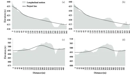
LiDAR data analysis for longitudinal sections

Fig. 4 shows the longitudinal sections of roads 1 and 2 taken by LTS and LiDAR. Project line has

been designed on these sections and indicates the fill and cut sections. In comparison to field-sur-veyed longitudinal sections by LTS, the LiDAR-derived sections exhibited elevation accuracy of 0.31 and 0.66 m for roads 1 and 2, respectively (Table 4).

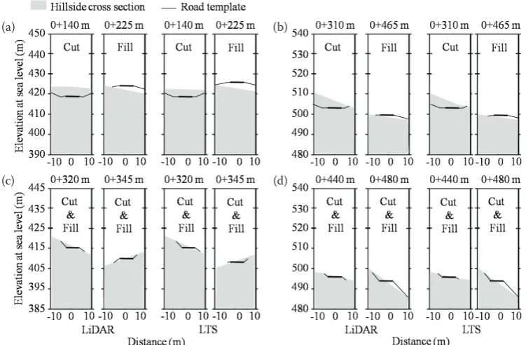
LiDAR data analysis for cut and fill volumes

Fig. 5 shows the samples of cut and fill areas af-ter assembly with road template on hillside cross sections. Cut and fill volumes were overestimat-

ed by the LiDAR for road 2 (134.47 and 91.47 m3_,

respectively), and underestimated for the cut vol-ume of road 1 (Table 5). In comparison to field-surveyed cross sections by LTS (placed every 5 m), the LiDAR-derived sections every 1 m

exhib-ited cut and fill accuracy of 2.39 and 3.18 m3 _for

road 1 and 2.98 and 5.60 m3 _{for road 2, respectively} (Table 6).

Table 3. Estimated elevation differences of cross sections between LiDAR detection and routes measured by Leica Total Station in the field

Proposed road

Points of the cross section (m)

upper middle lower

MD SD MD SD MD SD

Road 1 0.44 0.34 0.31 0.55 0.15 0.17 Road 2 0.50 0.51 0.66 0.53 0.63 0.39 MD – mean difference, SD – standard deviation

Fig. 4. Project lines on longitudinal sections taken by LiDAR (a, c) and Leica Total Station (b, d): road 1 (a, b), road 2 (c, d) Table 4. Estimated vertical alignment differences between LiDAR detection and routes measured by Leica Total Station in the field

Proposed road Elevation (m)

MD SD

Road 1 0.31 0.55

Road 2 0.66 0.53

MD – mean difference, SD – standard deviation

(a) (b)

LiDAR versus LTS

Differences between field-surveyed and LiDAR-derived horizontal, vertical alignments and earth-work volumes from 173 road points were compared using a paired t-test. A P-value of more than 0.05 in-dicated that the differences between LTS and LiDAR were not significantly different (Table 7).

Road 1 versus road 2

Table 8 shows the forest structure and terrain physiography properties of stands covered the pro-posed roads. Results showed that road 2 passed from difficult terrain with an elevation range of 492–505 m a.s.l. and hillside gradient of 20–50 %.

Fig. 5. Samples of cut and fill areas after assembly road template on hillside cross sections: road 1 (a, c), road 2 (b, d) LTS – Leica Total Station

Table 5. Cumulative cut and fill volume estimated by LiDAR and Leica Total Station (LTS)

Proposed road

Cumulative

cut volume (m3_{) fill volume (m}Cumulative 3₎

LTS LiDAR LTS LiDAR

Road 1 5,314.06 5,149.01 5,152.73 5,194.93 Road 2 8,899.57 9,034.04 8,724.37 8,815.84

Table 6. Estimated earthwork volume differences between LiDAR detection and routes measured every 5 m by Leica Total Station in the field

Proposed

road Cut (m

3_{) Fill (m}3₎

MD SD MD SD

Road 1 2.39 2.27 3.18 2.47

Road 2 2.98 3.75 5.60 5.36

MD – mean difference, SD – standard deviation

Table 7. t-Value and significant level in paired samples test of Leica Total Station and LiDAR

Proposed road Longitudinal section Horizontal alignment Cross section Earthwork volume

Road 1 –1.120ns _–1.499ns _–1.899ns _–1.648ns

Road 2 –1.128ns _–1.231ns _–0.175ns _–0.986ns

ns – not significant

Table 8. Forest structure and physiography properties of stands covered the proposed roads

Elevation (m a.s.l.) Hillside Volume (m3_·ha–1₎ Canopy cover (%) gradient (%) direction

Road 1 411–438 0–20 SW to NW 200–300 74

Road 2 492–505 20–50 W to NW 400–500 77

(a) (b)

Road 1 passed from an elevation range of 411 to 438 m a.s.l. and slope range of 0–20%. Moreover, road 2 was located under the dense stands with

trees volume of 400–500 m3 _{and canopy cover of}

77%. Accuracy differences between roads 1 and 2 were compared using a paired t-test. The difference in LiDAR accuracy between two roads was found to be statistically significant (P < 0.05, Table 9).

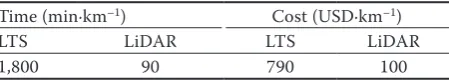
Time and cost expenditure for LTS and LiDAR

Time and cost comparisons are presented in Ta-ble 10 between LTS and LiDAR measurement. In this measurement, the time required for the LTS

was recorded as 1,800 min·km–1 _{which was 20 times}

more than that of LiDAR. The required total time

using LiDAR was 90 min·km–1_{. When comparing}

cost consumed for those two methods, there was

690 USD·km–1 _{difference to accomplish each task.}

DISCUSSION

In this study, the distance between the field-sur-veyed horizontal alignment and extracted align-ment from LiDAR was computed to yield MD and SD for each proposed road. The LiDAR-derived roads exhibited a positional accuracy of 0.23 and 0.47 m for roads 1 and 2, respectively. The road 2 showed the greatest difference with an average horizontal error of 0.47 m, which was considerably more than the road 1, which was located on gentle terrain and under the open canopy cover (Mayer et al. 2006; Clode et al. 2007). Azizi et al. (2014) developed a three-step classification approach for forest road extraction utilising LiDAR data. Results showed that the ±1.3 m positional accuracy for

road features is a substantial improvement com-pared to the accuracy (±10 m) of traditional data sources used to plot roads on the 1:25,000 topo-graphic maps in Iran. Craven and Wing (2014) used the airborne LiDAR to investigate the charac-teristics of forest roads under the different condi-tions of canopy cover. The vertical and horizontal error of LiDAR data in assessing central alignment of the road were 0.28 and 1.21 m, respectively. De-pending on the spatial resolution, some areas are difficult to identify due to minimal canopy penetra-tion (Mnih, Hinton 2012; Satio et al. 2013). If the lowest LiDAR return or high resolution DEM in an area is assumed, then the resulting topographic surface contain gullies, earth slumps, or hum-mocky topography will be easily identified since it will not look like a real ground surface (Robinson et al. 2010). In the current research, the horizon-tal alignment taken by LTS has some sharp turns, which makes it difficult for turning analysis. This problem is avoided by the LiDAR. Some research-ers reported that LiDAR data is a secure source in estimating longitudinal section and the position of central alignment of the road (Craven, Wing 2014; Hui et al. 2016).

Elevations for the road profile were extracted from the DEM along the road centreline (Saito et al. 2008). The examination of the vertical accuracy of the LiDAR data involved comparing field surveyed longitudinal section along the centreline of the road with elevations for the same horizontal position es-timated from the LiDAR-eses-timated DEM showed that vertical accuracy was lower in road 2. In com-parison to field-surveyed longitudinal sections by LTS, the LiDAR-derived sections exhibited eleva-tion accuracy of 0.31 and 0.66 m for roads 1 and 2, respectively. High standard deviations in horizontal and vertical alignment detection occurred where canopy density over the road was typically the great-est (Ziems et al. 2012). This made it more difficult on the analyst to determine the road location. Reute-buch et al. (2003) tested airborne LiDAR using 347 elevation points collected via LTS and GPS across four canopy classes: clear-cut, lightly thinned, heav-ily thinned, and uncut. Results showed the uncut site had the largest average error. Gomes-Pereira and Janssen (1999) reported a range of vertical

er-Table 9. t-Value and significant level in paired samples test of roads 1 and 2

Statistics Longitudinal section Horizontal alignment Cross section _cut Volume _fill

t-Value –5.334 –3.401 –8.865 –3.093 –5.518

Sig. (2-tailed) 0.000 0.001 0.000 0.003 0.000

Table 10. Estimated cost and time expenditure differences between proposed forest roads mapped by LiDAR and Leica Total Station (LTS)

Time (min·km–1_{) Cost (USD·km}–1₎

LTS LiDAR LTS LiDAR

ror values (0.08–0.15 m) on flat ground and larger errors on the sloped ground (0.25–0.38 m).

In comparison to field-surveyed cross sections by LTS, the LiDAR-derived sections exhibited cut

and fill accuracy of 2.39 and 3.18 m3 _{for road 1}

and 2.98 and 5.60 m3 _{for road 2, respectively. In}

general, it is noticed that the differences in earth-work volume estimates between LiDAR and LTS become larger as terrain ruggedness and canopy density increases (Xiao et al. 2017). Previous stud-ies conducted by Contreras et al. (2012) also highlighted the importance of canopy cover den-sity and terrain ruggedness in improving the ac-curacy of earthwork volume calculation, which is consistent with our findings in this study. While LiDAR is able to record details in terrain varia-tions by using 1 m cross section spacing, these terrain details are ignored when 5 m cross section spacing are considered in LTS. In this study, it was proved that the road project can be prepared faster by LiDAR than that of LTS.

CONCLUSIONS

Today total station and LiDAR laser scanner are used for many tasks in different applications such as geodesy, engineering, architectural and mining surveys with different accuracy level. We examined the accuracy of airborne LiDAR for forest road pro-jection across two stand structures. The obtained results from this study improved the knowledge about accuracy and time consumption of two sur-veying methods used (LTS and LiDAR). Based on the findings, with use of the LiDAR data, the accu-racy of vertical alignment and horizontal alignment and consequently earthwork volume increased as extracted point spacing is reduced to 1 m. The re-sults of this research indicated that the properties of proposed forest roads can be analysed rapidly under dense tree canopy using LiDAR data. The ac-curacy of road mapping using LiDAR can be used for quantitative terrain analysis without the need for ground reconnaissance in the field. LiDAR pro-vides the ability to analysis proposed roads on large scales in denied areas where the ground survey is not possible.

References

Akay A.E. (2006): Minimizing total cost of forest roads with computer-aided design model. Sadhana – Academy Pro-ceedings in Engineering Sciences, 31: 621–633.

Alharthy A., Bethel J. (2004): Automated road extraction from LiDAR data. In: Bethel J. (ed.): Proceedings of the American Society of Photogrammetry and Remote Sensing Annual Conference, Anchorage, June 23–24, 2004: 51–58.

Amo M., Martinez F., Torre M. (2006): Road extraction from aerial images using a region competition algorithm. IEEE Transactions on Image Processing, 15: 1192–1201. Azizi Z., Najafi A., Sadeghian S. (2014): Forest road

detec-tion using LiDAR data. Journal of Forestry Research, 25: 975–980.

Chekole S.D. (2014): Surveying with GPS, total station and terrestrial laser scanner: A comparative study. [MSc Thesis.] Stockholm, School of Architecture and the Built Environ-ment, KTH Royal Institute of Technology: 55.

Clode S., Rottensteiner F., Kootsookos P., Zelniker E. (2007): Detection and vectorization of roads from LiDAR data. Photogrammetric Engineering and Remote Sensing, 73: 517–535.

Coffin A.W. (2007): From roadkill to road ecology: A review of the ecological effects of roads. Journal of Transport Ge-ography, 15: 396–406.

Contreras M.A., Aracena P., Chung W. (2012): Improving ac-curacy in earthwork volume estimation for proposed forest roads using a high-resolution digital elevation model. Cro-ation Journal of Forest Engineering, 33: 125–134.

Coulter E., Chung W., Akay A., Sessions J. (2001): Forest road earthwork calculations for linear road segments using a height resolution digital terrain model generated from LiDAR data. In: Proceedings of the First International Precision Forestry Symposium, Seattle, June 17–20, 2001: 125–129.

Craven M., Wing M.G. (2014): Applying airborne LiDAR for forested road geomatics. Scandinavian Journal of Forest Research, 29: 174–182.

David N., Mallet C., Pons T., Chauve A., Bretar F. (2009): Path-way detection and geometrical description from ALS data in forested mountaneous area. The International Archives of the Photogrammetry, Remote Sensing and Spatial Informa-tion Sciences, XXXVIII (Part 3/W8): 242–247.

Espinoza F., Owens R.E. (2007): Identifying roads and trails hidden under canopy using LiDAR. [MSc Thesis.] Monterey, Naval Postgraduate School: 25.

Evans J.S., Hudak A.T., Faux R., Smith A.M.S. (2009): Discrete return LiDAR in natural resources: Recommendations for project planning, data processing, and deliverables. Remote Sensing, 1: 776–794.

Ferraz A., Mallet C., Chehata N. (2016): Large-scale road detection in forested mountainous areas using airborne topographic lidar data. ISPRS Journal of Photogrammetry and Remote Sensing, 112: 23–36.

Grote A., Heipke C., Rottensteiner F. (2012): Road network extraction in suburban areas. The Photogrammetric Record, 27: 8–28.

He Y., Song Z., Liu Z. (2017): Updating highway asset inven-tory using airborne LiDAR. Measurement, 104: 132–141. Hickerson T.F. (1964): Route Location and Design. New York,

McGraw-Hill: 634.

Hinz S., Baumgartner A. (2003): Automatic extraction of urban road networks from multi-view aerial imagery. ISPRSJournal of Photogrammetry and Remote Sensing, 58: 83–98.

Hui Z., Hu Y., Jin S., Yevenyo Y.Z. (2016): Road centerline extraction from airborne LiDAR point cloud based on hierarchical fusion and optimization. ISPRS Journal of Photogrammetry and Remote Sensing, 118: 22–36. Ichihara K., Tanaka T., Sawaguchi I., Umeda S., Toyokawa

K. (1996): The method for designing the profile of forest roads supported by genetic algorithm. Journal of Forestry Research, 1: 45–49.

Krogstad F., Schiess P. (2004): The allure and pitfalls of using LiDAR topography in harvest and road design. In: Nelson J., Clark M. (eds): Proceedings of the Joint Conference of IUFRO 3.06 Forest Operations in Mountainous Conditions and the 12th _{International Mountain Logging Conference,} Vancouver, June 13–16, 2004: 1–10.

Lacoste C., Descombes X., Zerubia J. (2005): Point processes for unsupervised line network extraction in remote sens-ing. IEEE Transactions on Pattern Analysis and Machine Intelligence, 27: 1568–1579.

Liu K., Sessions J. (1993): Preliminary planning of road systems using digital terrain models. Journal of Forest Engineering, 4: 27–32.

Mayer H., Hinz S., Bacher U., Baltsavias E. (2006): A test of automatic road extraction approaches. The International Archives of the Photogrammetry, Remote Sensing and Spatial Information Sciences, 36: 209–214.

Mena J., Malpica J. (2005): An automatic method for road extraction in rural and semi-urban areas starting from high resolution satellite imagery. Pattern Recognition Letter, 26: 1201–1220.

Mnih V., Hinton G. (2012): Learning to label aerial images from noisy data. In: Langford J., Pineau J. (eds): Proceedings of the 29th _{International Conference on Machine Learning,} Edinburgh, June 26–July 1, 2012: 203–210.

Reutebuch S.E., McGaughey R.J., Andersen H., Carson W. (2003): Accuracy of a high-resolution lidar terrain model under a conifer forest canopy. Canadian Journal of Remote Sensing, 29: 527–535.

Robinson C., Duinker P., Beazley K. (2010): A conceptual framework for understanding, assessing, and mitigating ecological effects of forest roads. Environment Reviews, 18: 61–86.

Saito M., Aruga K., Matsue K., Tasaka T. (2008): Development of the filtering technique of the intersection angle method using LiDAR data of the Funyu Experimental Forest. Jour-nal of the Japan Forest Engineering, 22: 265–270. Satio M., Goshima M., Aruga K., Matsue K., Shuin Y., Taska

T. (2013): Study of automatic forest road design model considering shallow landslides with LiDAR data of Funyu Experimental Forest. Croatian Journal of Forest Engineer-ing, 34: 1–15.

Sessions J., Wimer J., Costales F., Wing M. (2010): Engineering considerations in road assessment for biomass operations in steep terrain. Western Journal of Applied Forestry, 25: 144–153.

Sidle R.C., Ziegler A.D. (2012): The dilemma of mountain roads. Nature Geoscience, 5: 437–438.

Souleyrette R., Hallmark S., Pattnaik S., O’Brien M., Vene-ziano D. (2003): Grade and Cross Slope Estimation from LiDAR-based Surface Models. Ames, Midwest Transporta-tion Consortium, Iowa State University: 73.

Türetken E., Benmansour F., Andres B., Pfister H., Fua P. (2013): Reconstructing loopy curvilinear structures using integer programming. In: Le Borgne H., Moo Yi K., Kara-man S., Tron R., Khan S. (eds): Proceedings of the IEEE Conference on Computer Vision and Pattern Recognition, Portland, June 23–28, 2013: 1822–1829.

Umeda S., Suzuki H., Yamaguchi S. (2007): Considerations in the construction of a spur road network. Journal of the Japan Forest Engineering Society, 22: 143–152.

Veneziano D., Souleyrette R., Hallmark S. (2002): Elevation of LiDAR for highway planning, location and design. In: Zhou G., Kafatos M. (eds): Proceedings of the 15th _William T. Pecora Memorial Remote Sensing Symposium/Lands-atellite Information IV/ISPRS Commission I/FIEOS 2002 Conference, Denver, Nov 10–15, 2002: 10–22.

White R.A., Dietterick B.C., Mastin T., Strohman R. (2010): Forest roads mapped using LiDAR in steeps forested ter-rain. Remote Sensing, 2: 1120–1141.

Xiao L., Wang R., Dai B., Fang Y., Liu D., Wu T. (2017): Hybrid conditional random field based camera-LIDAR fusion for road detection. Information Sciences, 432: 543–558. Ziems M., Breitkopf U., Heipke C., Rottensteiner F. (2012):

Multiple-model based verification of road data. ISPRS Annals of the Photogrammetry, Remote Sensing & Spatial Information Sciences, I-3: 329–334.