A Framework for Pension Policy Analysis in Ireland:
PENMOD, a Dynamic Simulation Model
Tim Callan
†, Justin van de Ven
‡and Claire Keane
§Corresponding Author: Tim.Callan@esri.ie
* The model described here is based upon the NIBAX model architecture, as described in van de Ven (2011). We are grateful to Gerry Hughes and to Pete Lunn for helping to plug gaps in our knowledge. We are also indebted to several members of CSO staff for assistance: Tom McMahon, Pamela Lafferty, Marion McCann, Deirdre Cullen, and Shaun McLaughlin. Responsibility for any errors or obscurities rests with the authors. † Economic and Social Research Institute, Dublin. Email: tim.callan@esri.ie
‡ National Institute of Economic and Social Research, London. Email: jvandeven@niesr.ac.uk § Economic and Social Research Institute, Dublin. Email: claire.keane@esri.ie
ESRI working papers represent un-refereed work-in-progress by researchers who are solely responsible for the content and any views expressed therein. Any comments on these papers will be welcome and should be sent to the author(s) by email. Papers may be downloaded for personal use only.
A Framework for Pension Policy Analysis in Ireland:
PENMOD, a Dynamic Simulation Model
∗
Tim Callan
†, Justin van de Ven
‡& Claire Keane
§Abstract
This paper describes a structural dynamic microsimulation model of the household that has been developed to explore behavioural responses to pensions policy counterfactuals in Ireland. The model is based upon the life-cycle theory of behaviour, which assumes that individuals make their decisions to maximise expected lifetime utility, subject to expectations that are consistent with the prevailing decision making environment. The model is calibrated to match Irish survey data.
Key Words: Dynamic Programming, Savings, Labor Supply, Pensions
JEL Classifications: C51, C61, C63, H31
1
Introduction
Public policy towards both private pensions and state-provided pensions must be framed in a long-term
context. Decisions regarding participation in private schemes, and the extent of contributions thereto,
have implications which unfold over time. In defined contribution (DC) schemes, an individual’s pension
fund is built up over the working lifetime, and then drawn down in retirement. Government’s budget
constraint also leads to trade-offs between the level of the state pension, the age at which it becomes
payable, and the taxes required to finance it. Because of the essential dynamic elements in pension
contributions and payments, the impact of policy changes is not well captured by static models, which
take a “snapshot” of the impact at a point in time. While such models (including SWITCH, the ESRI
tax-benefit model) can provide some insights into the impact of pension-related policies, a fuller analysis
must take account of the complex interplay of forces over time.
The approach taken here is well established in the economic literature on pensions. Essentially,
our model (PENMOD) takes a representative cohort of individuals and simulates key elements of their
lifetime experience . This includes both economic elements such as labour market participation and
wages as they age as well as demographic elements (marriage, divorce, children, death). Crucially,
decisions regarding savings and pensions are also taken into account. Policy instruments in terms of
income tax and social welfare are also included.
∗The model described here is based upon the NIBAX model architecture, as described in van de Ven (2011). We are grateful to Gerry Hughes and to Pete Lunn for helping to plug gaps in our knowledge. We are also indebted to several members of CSO staff for assistance: Tom McMahon, Pamela Lafferty, Marion McCann, Deirdre Cullen, and Shaun McLaughlin. Responsibility for any errors or obscurities rests with the authors.
†Economic and Social Research Institute, Dublin. Email: tim.callan@esri.ie
The need to take into account a sequence of decisions over each individual’s full lifetime (up to the
age of 120) imposes a very strict discipline on the degree of detail that can be incorporated into the
model. Static models (such as SWITCH) can include a very high degree of detail in their description of
the tax and welfare system. Dynamic models (such as PENMOD) must use a broader brush, in order
to be able to provide greater depth in terms of the analysis over time. Thus, it is not a case of one class
of model being “better” than another; rather it is a question of different classes of model being more
suitable for different purposes.
A number of strategic simplifications are needed to ensure that the dynamic microsimulation model
captures key features of the tax/welfare and pension systems while remaining tractable. One major
simplification is that the model does not attempt to deal with public sector pensions, where the issues
which arise are of a different type. We focus instead on the private sector, where decisions regarding the
balance between contributions towards pension savings and the income in retirement are more subject
to the influence of economic and policy variables. Secondly, we focus on private sector employees rather
than the self employed. This is because the terms of retirement for the self employed often depend upon
the envisage income arising from ownership of a family business, or revenues arising from its sale that are
distinct from the pension system with which we are immediately concerned. Third, we do not attempt
to deal with issues of illness and longer-term incapacity to work. There are both state schemes (Illness
Benefit, Invalidity Pension, Disability Allowance) and private schemes (permanent health insurance)
which are geared towards dealing with income support for those unable to work. The issues arising are,
however, too complex to include when modelling the long-term evolution of incomes and pensions and
are therefore outside the scope of the present model. Simplifications of this type are common in the
international literature in this area.
As regards the pension regime itself, this is characterised by up to five different types of pension
scheme running in parallel. Each scheme takes a defined contribution form, where the approach adopted
is to allow for schemes of differing “quality”, with the probability of obtaining higher quality pensions
rising with income — details of the approach are set out in Section 2.3.
The remainder of the paper is set out in 7 sections as follows. First, a full description of the
characteristics that are reflected by the model, and the behavioural framework upon which it is based,
are provided in Section 2. Section 3 provides technical details of how the model generates behavioural
responses to policy change. The approach taken to calibrate the model against Irish survey data is
described in Section 4, and calibrated model parameters are reported in Sections 5 and 6. A brief
example of the type of policy analysis that can be conducted using the model is reported in Section 7,
2
Model Speci
fi
cs
The decision unit in the model is the nuclear family unit, defined as a single adult or partner couple and
their dependant children.1 The model divides the life course into annual increments, and can be used to
consider household decisions regarding: consumption, labour supply, the portfolio allocation of liquid
wealth between safe and risky assets, and private pension contributions. These decisions are simulated
on the assumption that households maximise expected lifetime utility, given their prevailing
circum-stances, preferences, and beliefs regarding the future. A household’s circumstances are described by
their age, number of adults, number of children, wage rate, liquid wealth, pension opportunities, private
sector pension rights, and time of death. The belief structure is rational, in the sense that expectations
are calculated on probability distributions that are consistent with the intertemporal decision making
environment.
Of the eight characteristics that define the circumstances of a household, seven can be considered
stochastic (relationship status, number of children, private sector pension scheme eligibility, private
sector pension rights, wage rates, liquid wealth, and time of death), and only age is forced to be
deterministic.
As a brief overview, the model permits:
• the adjustment of preferences over consumption, leisure, and bequests
• adjustment of the imposed liquidity constraints, which are defined both in terms of hard credit
limits and variable interest charges that depend on the debt to income ratios
• inclusion of uncertainty over relationship status (single or couple)
— provided that relationship status is considered to be uncertain, the number of children in a
household can also be modelled stochastically
• alternative options in regard to the nature of uncertainty associated with labour incomes, including
the possibility of receiving a low (zero) wage offer
• households to invest some of their liquid wealth in a risky asset
— the nature of the uncertainty associated with returns to the risky asset can also be altered
• households to choose their labour supply between discrete alternatives
• adjustment of a detailed tax and benefits structure
• private sector pensions
— contribution rates (and ultimately membership) can also be made a decision variable
— contribution rates (employee and employer) can be made stochastic
— the stochastic nature of the return to private pension wealth can be adjusted
This section begins by defining the assumed preference relation, before describing the wealth
con-straint, the simulation of pensions, and the processes assumed for the evolution of income and household
size.
2.1
The utility function
Expected lifetime utility of householdiat agetis described by the time separable function:
Ui,t =
1 1−1/γ
(
u
µ
ci,t θi,t
, li,t
¶1−1/γ
+
+Et
"
β1δ
Ã
φ1,tu
µ
ci,t+1
θi,t+1
, li,t+1
¶1−1/γ
+ (1−φ1,t)¡ζa+ζbw+i,t+1¢1−1/γ
!
+
+β1β2 T
X
j=t+2
δj−t
Ã
φj−t,tu
µ
ci,j θi,j
, li,j
¶1−1/γ
+ (1−φj−t,t)¡ζa+ζbwi,j+¢1−1/γ
!⎤
⎦ ⎫ ⎬
⎭ (1)
where 1/γ >0 is the (constant) coefficient of relative risk aversion; Et is the expectations operator; T is the maximum potential age; β1, β2, and δ are discount factors (assumed to be the same for all households);φj−t,tis the probability of living to agej, given survival to aget;ci,t∈R+is discretionary
composite consumption; li,t ∈[0,1] is the proportion of household time spent in leisure; θi,t ∈R+ is
adult equivalent size based on the “revised” or “modified” OECD scale; the parametersζaandζbreflect
the “warm-glow” model of bequests; andw+i,t ∈R+ is net liquid wealth when this is positive and zero
otherwise.
The labour supply decision (if it is included in the model) is considered to be made between discrete
alternatives, which reflects the view that this provides a closer approximation to reality than if it is
defined as a continuous decision variable for given wage rates. When adults are modelled explicitly,
then households with one adult can choose from up to three labour options; full-time¡lF T i,t
¢
, part-time
¡
lP T i,t
¢
, and not employed(li,t= 1). Similarly, couples can choose from up tofive labour options; both
full-time employed ¡l2i,tF T¢, one full-time and one part-time employed ¡lF tP ti,t ¢, one full-time and the other not employed¡lF tN ei,t ¢, one part-time and the other not employed¡lP tN ei,t ¢, and both not employed
(li,t = 1). When adults are not modelled explicitly, then labour supply is restricted to one of two
options: employed or not employed.
To the extent that the focus on discrete labour options limits employment decisions relative to
simulation model, and dampen variation in employment incomes. The former of these effects implies
that the parametrisation of the model may require a labour elasticity that overstates the practical
reality, while the latter suggests that excessive variation in labour incomes may be required to reflect
the wage dispersion described by survey data.
The modified OECD scale assigns a value of 1.0 to the household reference person, 0.5 to each
additional adult member and 0.3 to each child, and is currently the standard scale for adjusting before
housing costs incomes in European Union countries. Its inclusion in the preference relation reflects the
fact that household size has been found to have an important influence on the timing of consumption
(e.g. Attanasio & Weber (1995) and Blundell et al. (1994)).2
The model incorporates an allowance for behavioural myopia, through its assumption of
quasi-hyperbolic preferences following Laibson (1997). Such preferences are interesting because they are time
inconsistent, giving rise to the potential for “conflict between the preferences of different intertemporal
selves” (Diamond & Köszegi (2003), p. 1840). The current version of the model focuses exclusively
on rational expectations, and consequently does not permit consideration of decisions by so-called
“naïve” consumers, who are unaware of their self-control problems in the context of quasi-hyperbolic
discounting. The model assumes that all discount parameters are the same for all individuals, and time
invariant. This is in contrast to the approach that is adopted by Gustman & Steinmeier (2005), who
allow variation in the rate of time preference to be an important factor in reflecting heterogeneity in
household retirement behaviour. We have chosen not to do this to ensure that heterogeneity of household
behaviour generated by the model is driven by heterogeneity in observable household characteristics.
The warm-glow model of bequests simplifies the associated analytical problem, relative to
alterna-tives that have been considered in the literature.3 Including a bequest motive in the model raises the
natural counter-party question of who receives the legacies that are left. The most accurate
approxi-mation to reality would involve including the possibility that households receive a bequest at any age,
and then to growth adjust the value of bequests received to the value of bequests made. This would
add to the uncertainty associated with the decision problem, and so is omitted from the current version
of the model. Rather, it is assumed that households leave their legacies to the state (potentially in the
form of a 100% inheritance tax), which is a common simplifying assumption.
A Constant Elasticity of Substitution function was selected for within period utility,
u
µ
ci,j θi,j
, li,t
¶
=
õ
ci,j θi,j
¶(1−1/ε)
+α1/εl(1i,t−1/ε)
! 1
1−1/ε
(2)
2An empirical study by Fernandez-Villaverde & Krueger (2006) of US data from the Consumer Expenditure Survey suggests that roughly half of the variation observed for lifetime household consumption can be explained by changes in household size, as described by equivalence scales. See Balcer & Sadka (1986) and Muellbauer & van de Ven (2004) on the use of this form of adjustment for household size in the utility function.
whereε >0is the (period specific) elasticity of substitution between equivalised consumption(ci,t/θi,t)
and leisure (li,t). The constant α > 0 is referred to as the utility price of leisure. The specification
of intertemporal preferences described by equations (1) and (2) is standard in the literature, despite
the contention that is associated with the assumption of time separability (see Deaton & Muellbauer
(1980), pp. 124-125, or Hicks (1939), p. 261). This specification of preferences implicitly assumes that
characteristics which affect utility, but are not explicitly stated, enter the utility function in an additive
way.
2.2
The wealth constraint and simulation of disposable income
Equation (1) is considered to be maximised, subject to an age specific credit constraint imposed on
liquid net worth, wi,t ≥Dtfor household iat age t.4 The age profile of Dt can either be exogenously
defined in the model, or be relaxed subject to the constraint that all households must have repaid their
debts by an exogenously defined age, tD ≤T (the maximum terminal age assumed for the model).5
Liquid net worth is defined as the sum of safe liquid assets, ws
i,t ∈ [Dt,∞), and risky liquid assets, wr
i,t∈[0,∞). Intertemporal variation ofwi,t is described by: wi,t=
½
ˆ
wi,t t6=tSP A
(1−πl
a) ˆwi,t+ (1−πpa)w p
i,t+ (1−πoa)woi,t t=tSP A (3a)
ˆ
wi,t =
½
πdiv(wi,t−1−ci,t−1+τi,t−1) nat < nat−1, t < tSP A
wi,t−1−ci,t−1+τi,t−1 otherwise (3b)
τi,t=τ(li,t, xi,t, nai,t, nci,t, ri,ts wsi,t, rtrwi,tr , pci,t, t) (3c)
ln (1 +rtr)∼N
µ
μr− σ2r
2 , σ 2
r
¶
(3d)
where wpi,t denotes wealth held in personal pensions; woi,t is wealth held in occupational pensions; πla, πp
a, andπoaare, respectively, the proportions of liquid wealth, private pension wealth, and occupational
pension wealth that are used to purchase a life annuity at state pensionable age, tSP A; πdiv is the
proportion of liquid wealth that is assumed to be lost upon marital dissolution prior totSP A(to capture
the impact of divorce); andτ(.)denotes disposable income net of non-discretionary expenditure. As the model has been designed explicitly to undertake public policy analysis, particular care was
taken in formulating the module that simulates the effects of taxes and benefits on household disposable
incomes. Equation (3c) indicates that taxes and benefits are calculated with respect to labour supply,
li,t; private non-property income,xi,t; the numbers of adults,nai,t, and children,nci,t; the return to safe
liquid assets,rsi,twsi,t(which is negative whenwi,ts <0); the return realised on risky liquid assets,rrtwri,t
4Note thatw+
i,treferred to above is related towi,t, withw
+
i,t= 0ifwi,t<0, andwi,t+ =wi,totherwise.
(possibly negative); contributions to private sector pensions,pci,t; and age,t.
The form of the budget constraint described by equation (3a) has been selected to minimise the
computational burden of the utility maximisation problem. For the purposes of taxation, and in a
discrete time model such as this, investment returns can be calculated on the basis of wealth held at
the beginning of a given period, or wealth held at the end of the period. Calculating taxes with respect
to wealth held at the beginning of a period (as it is here) implies that disposable income is made
independent of consumption. This is advantageous when consumption is a choice variable, as it implies
that the numerical routines that search for utility maximising values of consumption do not require
repeated evaluations of disposable income for each consumption alternative that is tested.
We now describe details of the function that is used to evaluate disposable income. The lifetime is
divided into two periods for the purpose of calculating disposable income: the working lifetimet < tSP A,
and pension receipttSP A≤t. In each of these periods of life, household disposable income is calculated
by:
1. evaluating aggregatetake-home payfrom the taxable incomes of each adult member of a household
— this reflects the taxation of individual incomes in the Ireland
2. calculatingbenefits receipt from aggregate household take-home pay — this reflects the fact that
benefits tend to be provided at the level of the family unit
3. householddisposable income is then equal to aggregate take-home pay, plus benefits
Calculation of taxable income for each adult in a household depends on the household’s age, with
property and non-property income being treated separately. Prior to state pensionable age,t < tSP A,
household non-property income xi,t considered for tax purposes is equal to labour income gi,t less the
proportion of pension contributions that is considered tax exempt,πpe; from state pensionable age it is
equal to labour income plus the proportion of pension annuity income that is considered taxable,πpt: xi,t =
½
gi,t−πpepci,t gi,t+πptpi,t
t < tSP A
t≥tSP A (4)
where : pi,t=
(
χ(πpawpi,t+πlawˆi,t) t=tSP A
³ πs+(1
−πs).(na i,t−1)
πs+(1−πs).(na i,t−1−1)
´
pi,t−1 t > tSP A (5) pi,t denotes pension annuity income, and χ is the annuity rate considered for analysis. The annuity
purchased at agetSP Ais assumed to be inflation linked, and to reduce to a fractionπsof its (real) value
in the preceding year if one member of a couple departs the household in response to the mortality of
Where the household is identified as supplying labour, and is younger than state pensionable age,
then non-property (employment) income is split between spouses (in the case of married couples) on
the basis of their respective labour supplies. A household that is identified with a single wage earner
has all of its non-property income allocated to that one earner; a household with one full-time and
one part-time earner has non-property income allocated on the basis of an exogenously defined ratio;
and a separate ratio is used to divide non-property income when both spouses of a household are
full-time employed. A household without an employed adult has all of its non-property (pension) income
allocated to a single spouse.
Similarly, property income is only allocated between spouses for households below state pensionable
age, and who supply some labour. In this case, property income is allocated on the basis of an exogenous
ratio that defines the proportion of wealth that is assumed to be held in the name of the lowest earning
spouse. Property income, yi,t, is equal to the sum of returns from the safe and risky liquid assets:
yi,t=
⎧ ⎪ ⎪ ⎨ ⎪ ⎪ ⎩ rr
twri,t+rsi,twsi,t ifwsi,t>0;rrt >0 ri,ts wsi,t ifwsi,t>0;rrt ≤0
rr
twri,t ifwsi,t≤0;rrt >0
0 ifwsi,t≤0;rrt ≤0
(6)
Hence, the model assumes that the interest cost on loans, and losses due to negative risky asset returns
cannot be written offagainst labour income for tax purposes.
The interest rate on safe liquid assets is assumed to depend upon whether wi,ts indicates net invest-ment assets, or net debts:
rsi,t=
⎧ ⎨ ⎩
rI ifws
i,t>0 rlD+¡ruD−rlD
¢
min
½
−wi,ts max[gi,t,0.7g(hi,t,li,tf t)]
,1
¾
, rDl < rDu ifwi,ts ≤0
where lf ti,t is household leisure when one adult in household i at age t is full-time employed. This specification for the interest rate implies that the interest charge on debt increases from a minimum of
rD
l when the debt to income ratio is low, up to a maximum rate ofruD, when the ratio is high. The
specification also means that households that are in debt are treated less punitively if they have at least
one adult earning a full-time wage than if they do not.
The model is specified on the assumption thatrrt is distributed such thatμr< rlD, in which case no
rational (and risk averse) household will choose to borrow to fund investment in the risky liquid asset
(wr
i,t>0only ifwi,ts ≥0). Disposable income is consequently given by: τi,t =
⎧ ⎨ ⎩
ˆ
τi,t ifrtr≥0;wsi,t≥0
ˆ
τi,t+rrtwri,t ifrtr<0;wsi,t≥0
ˆ
τi,t+rstwsi,t ifwi,ts <0
(7)
ˆ
τi,t =
½
xi,t+yi,t−taxi,t+benef itsi,t−(1−πpe)
¡
pco i,t+pc
p i,t
¢
ift < tSP A
xi,t+yi,t−taxi,t+benef itsi,t−hsgi,t+ (1−πpt)pi,t ift≥tSP A (8)
2.2.1 Intertemporal indexing
It is likely that individuals take some account of wage growth when planning for the future: a 20 year
old today can reasonably expect that labour incomes will be higher when they reach age 45 than are
currently paid to today’s 45 year olds. If this is true, then it is important that the rational agent model
be calibrated against data that take wage growth into account (discussed at further length in Section
4). This gives rise to a host of complications regarding the appropriate intertemporal development to
assume for the tax and benefits system: holding taxes and benefitsfixed in the context of rising wages,
for example, will result in wide-spread tax bracket creep and marginalisation of the welfare state, with
important implications for simulated behaviour.
Two parameters of the model control the way in which the tax system evolve with time in the model.
Thefirst controls the rate at which tax thresholds grow with time, thereby offsetting bracket creep, and
the second controls the rate of growth of welfare benefits. These parameters adjust the tax and benefits
schedules in a way that is designed to omit the creation of poverty traps. Nevertheless, rapid temporal
adjustment of the tax system can give rise to analytical problems, and the the model is programmed
in a way that is designed to indicate when excessive variation has been called for. Separate routines
have been developed that allow the disposable income schedules that are generated by the model to be
viewed directly, and these are reviewed to verify that a model simulation is sensible.
2.3
Private Sector Pensions
Private sector pensions in the model are modelled at the household level, and are defined contribution in
the sense that every household is assigned an account into which their respective pension contributions
are notionally deposited. Although DC pensions account for less than half of all pensions that currently
attract contributions in Ireland, there has been a strong temporal trend toward DC schemes since
the 1990’s (in common with countries throughout the OECD), which motivates our modelling in this
regard. Up to five private sector pension schemes can be considered in parallel in the model, where
schemes are distinguished by their respective rates of (exogenously defined) employer contributions.
Pension contribution rates are defined as percentages of (total) labour income, implying that pension
membership requires employment participation. Households are considered to be eligible to participate
in only one pension scheme in any year, where eligibility to each scheme is identified stochastically with
reference to a set of income dependent probabilities, and uncertainty between adjacent years can be
suppressed in cases of continuous pension participation. Membership of a pension to which a household
is eligible can either be exogenously imposed, or modelled as an endogenous decision. Similarly, the
then these can be subject to a series of lower (πpl)and upper (πpu) bounds on eligible incomes, lower
(πpcl )and upper(πpc
u)bounds on contribution rates, and a ceiling on the value of the aggregate pension
pot,πp
max.
Accrued rights to a private pension are described by:
wpi,t =
½ ¡
1 +rtp−1¢wpi,t−1+¡πpi,t+πpec,j¢(gi,t−πpl)
¡
1 +rtp−1¢wpi,t−1
member of schemej
otherwise (9a)
ln (1 +rtp)∼N
Ã
μp−σ
2
p
2, σ 2
p
!
(9b)
2.4
Labour income dynamics
Up to three household characteristics influence labour income: the household’s labour supply decision,
the household’s latent wage, hi,t, and whether the household receives a wage offerwoi,t. Households
can be exposed to an exogenous, age and relationship specific probability of receiving a wage offer,
pwo¡na i,t, t
¢
. This facility is designed to capture the incidence of (involuntary) unemployment. If a
household receives a wage offer, then its labour income is equal to a fraction of its latent wage, with
the fraction defined as an increasing function of its labour supply. A household that receives a wage
offer and chooses to supply the maximum amount of labour receives its full latent wage, in which case
gi,t =hi,t. A household that does not receive a wage offer, in contrast, is assumed to receivegi,t = 0
regardless of its labour supply decision (implying no labour supply where employment incurs a leisure
penalty).
The decision to measure wage potential at the household level rather than at the level of the
individ-ual significantly simplifies the analytical problem. Separately accounting for the wages of each adult in
a household is properly addressed only by the addition of a state variable to the model where households
are comprised of an adult couple. Furthermore, there is significant empirical evidence to suggest that
men and women have quite different labour market opportunities, with those of women exhibiting a
relatively high degree of heterogeneity.6 Hence, accounting for the wage potential of individuals could
not ignore the sex of adult household members, thereby introducing an additional state variable. These
issues are further complicated by the difficulties involved in characterising sex-specific wage generating
processes, imperfect correlation of temporal innovations experienced by spouses, and so on. The model
side-steps these issues, as the current state of computing technology makes it impractical to address
them, and to analyse endogenous decisions over pension contributions.
In thefirst period of the simulated lifetime, t0, each household is allocated a latent full-time wage,
hi,t0, via a random draw from a log-normal distribution, log(hi,t0) ∼ N
¡
μna,t0, σ2na,t0
¢
, where the
parameters of the distribution depend upon the number of adults in the household, na. Thereafter,
latent wages follow a random walk with drift described by the equation:
log
Ã
hi,t m¡na
i,t, t
¢ !
= log
Ã
hi,t−1
m¡na
i,t−1, t−1
¢ !
+κ¡nai,t−1, t−1
¢(1−li,t−1)
(1−lW)
+ωi,t (10)
where the parametersm(.)account for wage growth (and depend on age,t, and the number of adults in the household,na
i,t),κ(.)is the return to another year of experience, andωi,t∼N
³
0, σ2
ω,na i,t−1
´
is a
household specific disturbance term.
A change in the number of adults in a household affects wages through the experience effect, κ, and the wage growth parameters m. This model is closely related to alternatives that have been developed in the literature (see Sefton and van de Ven, 2004, for discussion), and has the practical
advantage that it depends only upon variables from the current and immediately preceding periods
¡
t−1, na
i,t−1, nai,t, hi,t−1, li,t−1
¢
, which limits the number of characteristics that describe the
circum-stances of a household (and thereby the number of state variables in the optimisation problem).
Fur-thermore, although the concept of an experience term in a wage regression is well established7, its
inclusion is an innovation for the related literature (e.g. Low, 2005, and French, 2005). Most related
studies omit an experience term because it complicates the utility maximisation problem by invalidating
two-stage budgeting. We have, however, found that its inclusion enables us to better capture the profile
of labour supply during the life-course.
2.4.1 Complicating the standard decision making problem
The preferences defined by equations (1) and (2) are homothetic. Hence, if consumption and leisure
were each defined over a continuous domain, and if the price of leisure was exogenous, then the preferred
consumption to leisure ratio would be independent of an agent’s wealth endowment. In this case, within
period utility — equation (2) — at the decision making optimum can be expressed in terms of the period
specific measure of total expenditure (on goods and leisure), and the maximisation problem can be
resolved by two-stage budgeting. This decision making structure is fully consistent with the original
analysis of Arrow, so that interpretation of1/γas relative risk aversion (and, similarly, ofγas a measure of the intertemporal elasticity of substitution of total expenditure) carries over.8
However, the focus on discrete labour options, and the inclusion of an experience effect on wages,
complicate the intertemporal decision making problem. The discrete nature of labour supply implies
that it is not possible to restate intratemporal utility at the decision making optimum as a function
7With regard to statistical evidence of the effect of experience on income, Mincer & Ofek (1982) report that in the short run, every year out of the labour market can result in a 3.3%-7% fall in wages relative to those who remain employed. This study also finds, however, that the restoration of human capital tends to be faster than the original accumulation, so that the impact of early labour breaks reduce to 1.3%-1.8% in the long run. Eckstein & Wolpin (1989) do not make a distinction between the long run and short run impact of actual experience, butfind that thefirst year out of the labour market reduces wages by around 2.5%, with subsequent years having a marginally diminishing effect. See also, Waldfogel (1998) and Myck & Paull (2004) for the role of experience in explaining the gender wage gap.
of within period total expenditure. Nevertheless, optimised intratemporal utility remains a continuous
function of total within-period expenditure (albeit one that is subject to kinks at labour transitions) so
that it remains sensible to interpret1/γ as relative risk aversion (and, similarly,γ as a measure of the intertemporal elasticity of substitution of total expenditure). Meanwhile, the experience effect on wages
implies that the price of leisure is endogenous to the decision making problem, thereby invalidating two
stage budgeting. Furthermore, a positive experience effect on wages tends to depress savings rates as
wealth rises.9
2.5
Household composition
The model allows for households to form and to split, for the arrival of children, and for the risk of death
at different ages. The technical approach in terms of numbers of adults and children in a household is to
allow these to evolve stochastically, following a “reduced form” nested logit model. Thefirst (highest)
level determines the number of adults in a household, and the second (“nested” within that) determines
the number of children, given the age and number of adults in the household.
If the number of adults is selected to be uncertain, then a household can be comprised of either
a single adult or adult couple, subject to stochastic variation between adjacent years. The fact that
children typically remain dependants in a household for a limited number of years implies that it
is necessary to record both their numbers and ages when including them explicitly in the rational
agent model. This substantially increases the computational burden. If, for example, a household was
considered to be able to have children at any age between 20 and 45, with no more than one birth in
any year, and no more than six dependent children at any one time, then this would add an additional
334,622 state variables to the computation problem (with a proportional increase in the associated
computation time). In view of this, the model is currently specified to permit households to have up
to three children at each of two discrete ages, so that the maximum number of dependent children in a
household at any one time is limited to six.
This may seem somewhat artificial (it is as if larger families must involve multiple births, and births
only occur at two specific ages). The precise timing of births is not a centra focus of interest, however,
and the approach taken here means that the presence and number of children can be taken into account,
while abstracting somewhat from the associated detail.
The logit model that is considered to describe the evolution of adults in a household is given by
equation (11):10
si,t+1=αA0 +αA1t+αA2t2+αA3t3+αA4dki,t+αA5si,t (11)
where si,t is a dummy variable, that takes the value 1 if householdi is comprised of a single adult at
agetand zero otherwise, anddki,tis a dummy variable that equals 1 if householdiat agethas at least
one child. With regard to the simulation of births, four separate ordered logit equations are applied;
one for each of single and couple households, at each of the specified child-birth ages. The ordered
logit equations assumed for the first child birth age, for both singles and couples, do not include any
additional household characteristics. The ordered logit equations for the second child birth age includes
the number of children born at thefirst child birth age as an additional descriptive characteristic.
3
Solving the Life-time Decision Problem
This section begins by discussing the conceptual approach adopted to solve the lifetime decision making
problem, before describing details of the analytical routines used to implement the numerical solution.
3.1
Conceptual approach
The procedures that we adopt use backward induction to solve for decisions that maximise expected
lifetime utility. A terminal age T is assumed, following which death occurs with certainty. Utility maximising decisions at this terminal age are free of temporal dynamics, and are consequently
straight-forward to solve, for given numbers of adults nat, wealth wT, and annuity income pT, omitting the
household indexifor brevity. We refer to the utility associated with this solution as the value function,
VT(naT, wT, pT). Furthermore, we can calculate the intermediate measures of welfare:
b
u(naT, wT, pT) = u
µ b
cT(naT, wT, pT) θT
,1
¶
(12)
b
X(naT, wT, pT) = Et
µ
1 (1−1/γ)
¡
ζa+ζbwb+T+1(naT, wT, pT)
¢1−1/γ¶
(13)
where bcT and wbT+1 denote the optimised measures of consumption and next period wealth, on the
assumption that labour supply at the terminal age is not possible. We calculate these functions at all
nodes of a three dimensional grid in the number of adults, wealth, and retirement annuity.
At ageT−1, suppose that households are permitted to invest in risky assets and to supply labour. Here, the problem reduces to solving the Bellman equation:
VT−1(naT−1, wT−1, hT−1, woT−1, pT−1) = max
cT−1,νT−1,lT−1
(
1 1−1/γu
µ
cT−1
θT−1
, lT−1
¶1−1/γ
+
+ET−1
∙
β1δ
1−1/γ
³
φ1,T−1ub(naT, wT, pT)1−1/γ+ (1−φ1,T−1)
¡
ζa+ζbw+T¢1−1/γ´+ +β1β2δ2φ1,T−1Xb(naT, wT, pT)
io
(14)
subject to the intertemporal dynamics that are described above, wherewoT−1 is a wage offer identifier
taking the value 1 if a wage offer is received and zero otherwise, andνT−1 is the proportion of liquid
wealth invested in the risky asset. We solve this optimisation problem for theT−1value function, at each node of the five dimensional grid over the permissable state-space. The expectations operator is
evaluated in the context of the log-normal distributions assumed for wages and risky asset returns, using
the Gauss-Hermite quadrature, which permits evaluation at a set of discrete abscissae. Interpolation
methods are used to evaluate the value function at points between the assumed grid nodes throughout
the simulated lifetime.
Solutions for earlier ages then proceed via recursive repetition of the procedure outlined for ageT−1, given the solutions (previously) obtained for later ages. Prior totSP A, solutions may also be required
for pension contributions, and the state space may be expanded to include children and the pension
assets permitted in the model. A more complete description of the analytical problem, including the
treatment of boundary conditions, is reported in the technical appendix.
The above procedure generates a grid that spans all possible combinations of characteristics that the
model considers a household might have (the state space). The utility maximising decisions identified by
the numerical procedure are stored at each grid intersection, alongside the numerical approximation of
expected lifetime utility (the value function). Although this set of information can be informative in its
own right, most analyses are based upon panel data for the life-course of a cohort of households that are
generated using the grid defined above. The life course of a birth cohort is generated byfirst populating a
simulated sample by taking random draws from a joint distribution of all potential state variables at the
youngest age considered for analysis. The behaviour of each simulated household,i, at the youngest age is then identified by reading the decisions stored at their respective grid co-ordinates. Given household
i’s characteristics (state variables) and behaviour, its characteristics are aged one year following the processes that are considered to govern their intertemporal variation. Where these processes depend
upon stochastic terms, random draws are taken from their defined distributions (commonly referred to
3.2
Details of solution routines
The model described here is complex and generates behaviour where no analytical solution exists. As
such, it is reasonable to describe it as a ‘black-box’ routine, which raises concerns over the accuracy of
the behavioural responses that it generates. These concerns are exaggerated by the fact that the value
function may be both non-smooth and/or non-concave (although it is designed to be increasing and
continuous), which can complicate the solution due to the existence of multiple local maxima.
It is important to recognise from the outset that any numerical solution is likely to be associated
with a degree of error — the problem is to assess whether the scale of the inaccuracies generated by
the model are qualitatively important for the purpose to which it is applied. The model includes three
principal tools for assessing the accuracy of the numerical solutions that it derives: variation of solution
detail, variation of interpolation methods, and variation of the numerical search routines that are used.
Thefirst is the most simple, and often the most powerful of the three. Whenvarying the solution detail,
the size and number of grid points adopted for each of the continuous state variables can be altered, as
can the number of abscissae used in the Gaussian quadrature.11 Increasing the grid points provides a
more detailed solution of the utility maximising problem, though it can also imply a rapid increase in
computational burden. Increasing the grid points in multiple dimensions increases the computational
burden geometrically rather than arithmetically; a problem that is commonly referred to as the curse
of dimensionality.
The model includes both linear and cubic interpolation methods, for evaluating behaviour between
discrete grid points.12 Relative to linear interpolation, cubic interpolation produces a smoother
func-tional form, and ensures continuous differentiability. Cubic interpolation also requires evaluations at4n
grid points, rather than2n points, wheren is the number of dimensions over which the interpolation
is being taken. If the user indicates that cubic interpolation is to be used, then the model performs
an internal check to determine whether the surface over which an interpolation is being conducted is
reasonably smooth, before selecting the cubic interpolation for analysis; otherwise, it selects the linear
interpolation.13 It is of note that the cubic interpolation, and linear interpolation routines have been
programmed separately, and so can be used to validate against one another.
Finally, the model includes three alternativenumerical search routines, which are used tofind utility
maximising values of consumption. A ‘brute force’ procedure uses grid search methods to identify a
local optimum. The advantage of this approach is that it makes no assumptions regarding the form that
1 1Evaluation of weights and abscissae of the Gauss-Hermite quadrature are based upon a routine reported in Chapter 4 of Press et al. (1986).
1 2The interpolation routines that are used are based on Keys (1981).
the value function takes. This advantage is, however, purchased at a very substantial increase in the
computational burden associated with the search routine. Alternatively, Brent’s method can be used to
search over the consumption domain, based upon parabolic interpolation with a golden section search
of repeated evaluations of the value function. This approach has been found to be efficient, particularly
where the surface over which the search is conducted is reasonably well behaved, but is not designed
to take account of multiple local optima. The third search alternative is based upon the Bus & Dekker
(1975) bisection algorithm, which can be used to identify the consumption that evaluates the Euler
condition to zero. Like Brent’s method, the Bus & Dekker (1975) algorithm is recognised as efficient,
and is not designed to account for multiple local optima. Relative to Brent’s method, optimisation
of the Euler condition can — in some circumstances — result in improved accuracy, but at the cost of
increased computational burden (as repeated calls to the value function do not require the additional
computational burden involved in evaluatingfirst derivatives). Furthermore, some analytical contexts
may argue against the use of Euler conditions, as in the case where non-exponential discounting is
assumed.
Asupplementary search routineis included in the model to mitigate concerns regarding identification
of multiple local optima where Brent’s method or the Bus & Dekker algorithm are applied. Here the
model can be directed to explore a localised grid above and below an identified optimum for a preferred
level of consumption, based upon value function calls. If an alternative value of consumption is identified
by this supplementary routine as strictly preferred to the original local maximum, then the routine will
search recursively for any further solutions above and below. This process is repeated until no further
solutions are found. Of all feasible solutions, the one that maximises the value function is selected.
4
Data and Calibration Methodology
4.1
Data considered for calibrating the model
Cross-sectional data for Ireland observed in 2005 were primarily considered for calibrating the model.
This focus on cross-sectional data was adopted after careful consideration, taking into account the
lim-itations of the structural model and the primary purpose for which the model has been devised. The
model is limited in the sense that it does not capture real-world uncertainty over a range of
charac-teristics, including the evolving tax and benefits system, conditions of the macro-economy, household
demographics, and so on. As such, calibrating the model to survey data reported for a population birth
cohort requires the implicit assumption that either changes in the policy environment have an incidental
impact on behaviour, or are perfectly foreseen. The former of these assumptions is difficult to maintain
latter is patently inaccurate. Cross-sectional data avoid these problems because they describe behaviour
observed under a single policy environment. The assumptions implicit in the calibration are then that:
a) individuals base their decisions on the belief that the existing policy environment will be maintained
into the indefinite future; and b) that expectations regarding the future evolution of individual specific
characteristics — including demographics, wages, employment opportunities, and so on — can be based
upon age profiles exhibited by contemporary survey data. The former of these assumptions appears to
us to be plausible (if not necessarily accurate), as does the latter after an allowance is made for trend
improvements in wages and survival probabilities. These underlying assumptions should be borne in
mind when interpreting the discussion that follows.14
4.2
Calibration approach
The model was calibrated to survey data in a two stage process that adapts to the limitations of
available survey data and processing power, in common with most empirical studies based upon dynamic
programming techniques (e.g. (Gourinchas & Parker 2002)). In thefirst stage, estimates for observable
model parameters were calculated. Given the estimates obtained in the first stage, values for the
unobserved parameters of the model were adjusted in the second stage to match the moments for a
simulated cohort (described in Section 3) to sample moments estimated from survey data.
4.2.1 Specification of the model considered for calibration
As the second stage of the calibration requires testing over a very large number of parameter
combina-tions, the model was limited to the following eight characteristics:
- age - number of adults - wage offers - wage rates
- net liquid assets - pension eligibility - pension rights - time of death
This restricted model focuses on decisions over labour supply (including the possibility of part-time
employment), consumption, and pension participation, given a household’s age, its number of adults,
liquid assets, wage offer, wage rate, pension scheme eligibility, pension wealth, and survival. Household
decisions were considered at annual intervals between agest0 = 20 andT = 120, with labour supply
possible to age 75. State Pensionable Age was set to tSP A = 65, the pensionable age that prevailed
in 2005. Uncertainty was taken into consideration for the intertemporal development of the number of
adults in a household, wage offers, wage rates, private pension eligibility, and the time of death — age,
liquid wealth, and pension wealth were all considered to evolve deterministically.
As noted above, the model solves decision making problems by dividing the permissable state space
(the range of characteristics that any household might conceivably have) into a series of grids. The
domains of wages and wealth between ages 20 to 69 were each divided into 34 points using a log scale.
The domain of pension wealth between ages 20 to 64 was divided into 16 points using a log scale. It was
assumed that 25% of pension wealth at aget=tSP A is taken as a tax free lump, with the remainder
taken as a retirement annuity. The domain of the retirement annuity was divided into 16 points using a
log scale between ages 65 and 75. From age 76 to age 120, the wealth and retirement annuity domains
were each divided into 151 points using a log scale.
Three additional dimensions — reflecting the number of adults in a household, wage offers, and
pension scheme eligibility — complete the grids that were considered for the calibration. These grid
dimensions differ from those described above in that they refer to characteristics that take discrete
values. From age 20 to 95 (inclusive), solutions were required for single adults and couples; from age
96 all households were considered to be comprised of a single adult. Between ages 20 and 75, solutions
were required for households with and without a wage offer. Furthermore, 3 private sector pension
schemes were considered for analysis.
This specification of the model required utility maximising decisions to be numerically evaluated for
12,283,729 different combinations of household characteristics, for each alternative parameter
combina-tion tested as part of the calibracombina-tion process.15 For reference, this specification of the model takes 25
minutes to run on a computer with an Dell T5500 workstation with dual Xeon X5650 processors and
6Gb of RAM.
4.2.2 Calibration strategy
The parameters of the model that were not estimated on observable data (or otherwise exogenously
assumed) were calibrated by comparing age profiles at the household level for both singles and couples
of:
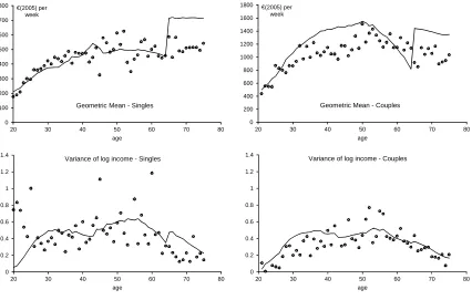
1. the geometric mean of household employment income
2. the variance of household log employment income
3. the proportion of adult household members employed full-time, part-time and not at all
4. the geometric mean of household consumption
5. the variance of household log consumption
Statistics on employment were derived from SILC 2005. Proportions employed full-time, part-time
or not in work were derived from the Quarterly National Household Survey (April 2005), while statistics
on consumption expenditure were derived from the Household Budget Survey, again for 2004/2005.
Age specific geometric means of household employment income were matched by altering the
distri-bution mean of the simulated cohort at entry to the model (age 20),μna,t
0, and by adjusting the age
and relationship specific trend parameters of human capital described bym¡na i,t, t
¢
in equation (10).
The variance of log employment income by age and relationship status was matched by adjusting the
variance of the distribution at entry to the model, σ2
na,t0, and the variance of age specific innovations,
σ2
ω,na
i,t−1. Age and relationship specific rates of employment participation were matched by adjusting the utility price of leisure,α, the learning by doing effects, κ¡ni,ta−1, t−1¢. Learning by doing effects,
κ¡na
i,t−1, t−1
¢
were also adjusted to match the model to the split between full-time and part-time
employment described by survey data, as were the ratios of part-time to full-time wages. Finally, the
timing of consumption was adjusted by altering the exponential discount rate δ, and the parameter of relative risk aversion 1/γ. The variance of consumption by age was a residual that depends heavily upon the associated income parametersnσ2
na,t0, σ2ω,na i,t−1
o
.
It was necessary to select a set of starting values for the model from which to commence the
calibration process. Starting with the wage parameters, we began with aflat wage profile over the life
course, assuming zero experience effects, κ= 0, and no risk of a low wage offer. The leisure cost of full-time and part-time employment were defined as non-stochastic and age invariant proportions of the
total time available to an adult, assuming 18 ‘viable’ hours per day. Similarly, the ratio of the part-time
to full-time wage was assumed to be independent of age and relationship status. The initial ratios
considered for the calibration were calculated using data from the 2005 wave of the SILC; associated
statistics are reported in Table 1. Finally, the preference parameters of the model were taken from UK
econometric regressions (see (van de Ven 2010)), but the search routine meant that parameters were
free to vary in response to characteristics in the Irish data. The exception is the utility price of leisure,
which was set deliberately low to ensure an adequate sample for calculating moments of employment
income.
The model calibration was conducted using a cascading procedure designed to subject the most
flexible aspects of the model to the most frequent instances of re-adjustment. From the list of moments
referred to above, the model exhibits the greatest degree offlexibility in relation to the geometric means
of household employment income, where the number of associated model parameters©μna,t
0, m
¡
na i,t, t
¢ª
is identical to the number of moments considered for the calibration. The calibration consequently
focussed in thefirst instance upon adjusting the parameters©μna,t0, m
¡
na i,t, t
¢ª
until a close match was
Given the calibrated parameters for employment income, the calibration focussed next upon
match-ing the incidence of employment participation / non-employment. Here, the utility price of leisure α
serves to reduce the preference for employment in general, and the learning-by-doing effectsκincrease employment early in the working lifetime, relative to later life. The parameter adjustments necessary
to match the model to employment participation, also serve to distort the match obtained to labour
income, both through the direct effect that varying the parametersκhave on the intertemporal devel-opment of latent full-time wages, and indirectly through distributional heterogeneity in labour supply
responses to employment incentives. Hence, the calibration process proceeded in an iterative loop to
match the model to both the geometric mean of employment income and employment participation at
the same time.
The calibration procedure focussed next upon matching the model to rates of full-time and
part-time employment. This aspect of the calibration proceeded in a very similar fashion to that set out for
employment participation, with the ratio of part-time to full-time wages replacing the utility price of
leisure in the adjustment of parameters. It is important to note that this adjustment procedure has the
very significant advantage that the wage parameters derived via the calibration take full account of the
endogeneity of labour supply decisions, with which so much of the associated econometric literature has
been concerned following the seminal contribution by James Heckman.
Having obtained a close match to moments of both employment income and labour supply, the
calibration then focussed upon matching the model to sample moments of household consumption. The
model offers relatively blunt tools with which to achieve this match, and the associated calibration is
somewhat more approximate as a result — in particular, we focussed upon achieving a match between the
peaks in consumption described by the simulated and sample data, and the general trend of age specific
variances in consumption. In this regard, the discount rate δ tends to shift consumption into later periods of life, increasing the slope of the lifetime consumption profile. The parameter of relative risk
aversion1/γ motivates increased precautionary saving early in the working lifetime, which diminishes as the working lifetime proceeds. An alternative aspect that has been recognised as important here
is the bearing that demographic needs have on consumption preferences; this aspect of the model was
omitted from the calibration, due to the exogenous assumption of age specific demographics (reported
in Section 5.4), and the revised OECD equivalence scale upon which the preference relation is based.
To summarise, the model parameters ©μna,t
0, m
¡
na i,t, t
¢ª
were then adjusted until a close match
was obtained to the age and relationship specific geometric means for employment income. Given the
parameters ©μna,t
0, m
¡
na i,t, t
¢ª
, the model parameters©α, κ¡na
i,t−1, t−1
¢ª
and the ratio of part-time
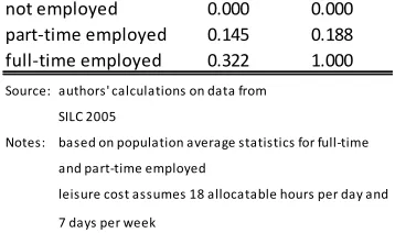
Table 1: Model Parameters to Distinguish the Effects on Leisure and Labour income of Alternative Labour Supply Decisions
employment option leisure
cost
propn of full‐ time wage
not employed 0.000 0.000
part‐time employed 0.145 0.188
full‐time employed 0.322 1.000
Source: authors' calculations on data from
SILC 2005
Notes: based on population average statistics for full‐time
and part‐time employed
leisure cost assumes 18 allocatable hours per day and
7 days per week
was then repeated a number of times until the model obtained a reasonable match to both geometric
means for employment income and rates of employment at the same time. The parameters{δ,1/γ}were then adjusted to to obtain a better match to age specific geometric means for consumption described by
survey data, and the parametersnσ2na,t0, σ2ω,na i,t−1
o
were adjusted to obtain an improved match to the
age specific moments of both consumption and labour income. The entire process was then repeated
to obtain the calibrated results that are reported in Section 6.
5
Estimates for Observable Parameters
The model parameters for which exogenous estimates were obtained are principally concerned with
four key issues: life expectancy, the terms of the available pension schemes, taxation, and household
demographics. A conspicuous omission from this list is the treatment of wages, the parameters for
which were addressed as part of the second stage calibration to ensure the approach taken to account
for sample selection is consistent with the wider analytical framework. The specification of these five
aspects of the model are described in turn below.
5.1
Life expectancy
The survival probabilities assumed for calibrating the model are based upon CSO Population and Labour
Force Projections, 2006-2036. These data are based upon observed survival rates between 2006 and
2007, and Official projections for improved longevity thereafter. The Official data permit survival rates
to be calculated to age 99. Age specific survival probabilities between 100 and 120 were exogenously
specified to obtain a smooth sigmoidal progression from the official estimate at age 99 to a 0% survival
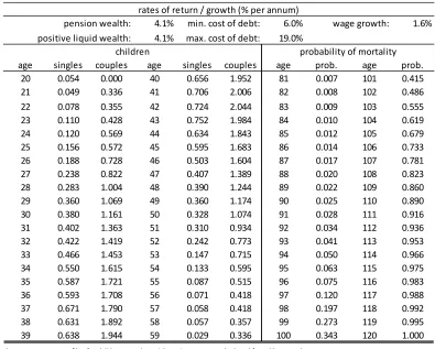
Table 2: Exogenously estimated model parameters
rates of return / growth (% per annum)
pension wealth: 4.1% min. cost of debt: 6.0% wage growth: 1.6%
positive liquid wealth: 4.1% max. cost of debt: 19.0%
children probability of mortality
age singles couples age singles couples age prob. age prob.
20 0.054 0.000 40 0.656 1.952 81 0.007 101 0.415
21 0.049 0.336 41 0.706 2.006 82 0.008 102 0.486
22 0.078 0.355 42 0.724 2.044 83 0.009 103 0.555
23 0.110 0.428 43 0.752 1.984 84 0.010 104 0.619
24 0.120 0.569 44 0.634 1.843 85 0.012 105 0.679
25 0.156 0.572 45 0.595 1.683 86 0.014 106 0.733
26 0.188 0.728 46 0.503 1.604 87 0.017 107 0.781
27 0.238 0.822 47 0.407 1.389 88 0.020 108 0.823
28 0.283 1.004 48 0.390 1.244 89 0.022 109 0.860
29 0.360 1.069 49 0.360 1.174 90 0.025 110 0.890
30 0.380 1.161 50 0.328 1.074 91 0.028 111 0.916
31 0.402 1.363 51 0.310 0.934 92 0.034 112 0.936
32 0.422 1.419 52 0.242 0.773 93 0.041 113 0.953
33 0.466 1.453 53 0.147 0.715 94 0.050 114 0.966
34 0.550 1.615 54 0.133 0.595 95 0.063 115 0.975
35 0.587 1.721 55 0.087 0.515 96 0.075 116 0.983
36 0.593 1.708 56 0.071 0.418 97 0.120 117 0.988
37 0.671 1.790 57 0.058 0.418 98 0.197 118 0.992
38 0.631 1.892 58 0.057 0.357 99 0.273 119 0.995
39 0.638 1.944 59 0.029 0.336 100 0.343 120 1.000
Source: age profiles for children equal to arithmetic averages calculated from ** survey data
mortality probabilities calculated for couples where both members are aged 20 in 2005 on life‐tables published ***
return to pension wealth and positive balances of liquid wealth set equal to real growth observed for Irish GNP between
1970 and 2005
cost of debt exogenously assumed
5.2
The terms of private sector pension schemes
The terms of private sector pensions in Ireland are complex and diverse (see, for example, thePension
Market Survey 2007, IAPF). Defined benefit schemes remain important, but in the private sector, and
especially for younger workers, defined contribution schemes have become much more common. In
order to summarise Irish private sector pensions in a tractable fashion, we have opted to characterise
the system in terms of a set of pension options which a worker may face. We represent DB schemes in
terms of a DC scheme with a higher employer contribution — this helps to capture a key feature of DB
schemes, while at the same time keeping the complexity of the problem to a manageable level.16
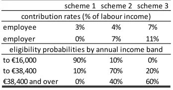
Three schemes are considered for the calibration, designed to reflect low, middle, and high pension
contribution rates by employees and their employers. Employees are considered to be able to decide
over whether to participate in these schemes, but not their respective rates of pension contributions, as
is common for occupational pensions. The terms applied to each of the representative pension schemes
are summarised in Table 3.
The top panel of Table 3 reports the rates of employee and employer pension contributions assumed
for each alternative pension scheme. In each year between ages 20 and 64, households are allocated a
pension scheme that they may choose to participate in during the respective year. The pension scheme
to which a household is eligible in any given year is either carried over from the scheme that they chose
to participate in during the preceding year, or — if they chose not to participate in a pension during the
preceding year — then it is taken as a random draw with reference to the income specific probability
distributions reported at the bottom panel of Table 3.
The statistics that are reported in Table 3 reflect the stylised observation that employer pension
provisions tend to improve with employee wages, where pension support is virtually non-existent for
employees on low wages — defined here as those with full-time wages worth less that €16,000. In
contrast, many employees toward the top of the wage distribution tend to enjoy relatively generous
pension support from their employers, while the majority of workers lie between these two extremes.
Furthermore, we ignore associated decisions regarding the portfolio allocation, and assume that all
returns to investment are risk free. The rate of return to pension wealth is set to 4.1% per annum,
equal to the average real growth of Gross National Product in Ireland during the period 1970 to 2005
(reported in the top panel of Table 2). Pension wealth is converted into an actuarially fair annuity
at age 65 based on the assumed rate of return to pension wealth and the mortality rates discussed in
Section, 5.1. The value of this annuity is assumed to falls by 50% upon the death of a spouse.
Table 3: Terms Assumed for Private Sector Pensions: contribution rates and probabilities of eligibility
scheme 1 scheme 2 scheme 3 contribution rates (% of labour income)
employee 3% 4% 7%
employer 0% 7% 11%
eligibility probabilities by annual income band to €16,000 90% 10% 0% to €38,400 10% 70% 20% €38,400 and over 0% 40% 60%
Notes: authors' assumptions for terms of private sector pensions
real return to pension wealth set to 4.1% p.a.
income thresholds for probability distributions indexed to
real wage growth of 1.6% p.a.
5.3
Taxes and bene
fi
ts
We adopt a simplified representation of the tax/welfare system, which nevertheless captures some of
the key features of interest. For the cohorts now entering the labour market, coverage of the State
Contributory Pension scheme will be much higher than heretofore. We consequently adopt the
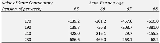
simpli-fying assumption that, in future, all those aged above State Pension Age will be eligible for the State
Contributory Pension. The model allows for both the State Pension Age and the level of payment to
be varied.
For those of working age, we take account of the following schemes:
• Jobseekers’ Allowance
• One Parent Family Payment
• Child income support via child benefit, qualified child increase and Family Income Supplement
On the income tax side, we allow for the basics of personal and PAYE tax credits, tax bands
and rates, and for PRSI and levies (which may be structured along the lines of the Universal Social
Charge). Special attention is given to alternative possible tax treatments of pensions, varying from
the EET (exempt, exempt, taxed) structure which approximates that in place until recent years to a
potential new system with tax relief at a single hybrid rate, as per the recommendations of the National
Pension Framework.
An additional issue of concern in relation to the simulated tax and benefits system is the way that
it is assumed to evolve with time. Given the wage growth that is used to adjust thefinancial statistics
against which the model is calibrated (reported in Section 4), ignoring indexation would result in “fiscal
drag” (or tax bracket creep) and a decline in the relative value of benefits. Three main approaches
payment levels with respect to wage growth. This has the merit of ensuring that the ratio of tax to
income remains constant, and that welfare incomes rise in line with general wage growth. This approach
is in line with the distributionally neutral benchmark adopted in analysis of budgetary impact.
An alternative approach would be to project indexation of tax parameters and of wel