On Resolving Ambiguities in Arbitrary Shape extraction by the HT

Invariant Characterization of the

Hough Transform for Pose

Estimation of Arbitrary Shapes

Alberto S. Aguado

1

, Eugenia Montiel

2

and Mark S. Nixon

3

1

Electronic Engineering, University of Surrey, UK

2

iMAGIS, INRIA Rhône-Alpes, France

3

University of Southampton, UK

Abstract

We develop a new formulation for including invariance in a general form of the Hough transform. We first develop a formal definition of the Hough transform mapping for arbitrary shapes and general transformations. We then include an invariant characterization of shapes and we develop and apply our technique to extract shapes under similarity and affine transformations. Our characterization does not require the computation of properties for lines or other primitives that compose a model, but is based solely on the local geometry given by points on shapes. Experimental results show that the new technique is capable of extracting arbitrary shapes under occlusion and when the image contains noise.

1

Introduction

In shape extraction, it is important to be able to handle difference in an object’s appearance due to change in camera position [1]. Some techniques, including cluster methods, pose clustering, evidence gathering, geometric hashing and hypothesis accumulation have handle changes in object’s appearance by verifying the consistency between structures in the image and in the target shape [2-6]. Our approach circumvents this problem by including invariant properties within the evidence gathering procedure of the Hough transform (HT). Our formulation is focused on similarity and affine transformations and it avoids problems due to the uncertainty in the location or lines and other image primitives [7] by considering only edge points in a shape. We take as our starting point the evidence gathering of Fourier parameterized shapes [8]. The use of parameterized shapes ameliorates difficulties inherent in use of tabular curve descriptions (as in the Generalized Hough transform (GHT)).

2

Evidence gathering of arbitrary shapes

Model shape extraction is fundamentally a problem of analysis of regression [9]. Here, we consider as a fitting curve a parametric model defined by a shape model υ( )s and a parametric transformation fa. Thus, a parametric model is defined as

( )s,a f(a,υ( )s )

model shape w ,( )s a is relative to the origin. Therefore, a primitive in an image is represented by a translation of the model. That is,

( )a w( )a b

z s, = s, + (1)

where the point b=(a0, b0) defines the position of the primitive in an image. The shape extraction problem is solved by determining the parameters in a and the position b such that they define a curve z ,

( )

s a that best fits the image data. Deviations due to the use of minimization of quadratic errors combined with the change in the position of the objects have been discussed in [10,11].

The Hough transform (HT) obtains a robust mode fitting by gathering evidence of all the potential values of the parameters defined when a point in an image is matched to a point in the model. For eq. (1), if a point in an image λ0 is matched to a point in the model z

( )

s₀,a , then the location parameter as a function of λ0 and ais given by

( 0,a) (ba0,b0)

bλ = (2)

for b(λ0,a)= λ0−w(s0,a). That is, the location can be determined given a point in the image and the parameters of the transformation. Each combination of the parameters defines a potential value for the location. That is, the match of a point in the model and a point in the image defines a hyper-surface in the parameter space. This hyper-surface defines the point spread function (psf) of the pointλ0. In the HT, the parameters are computed by increasing the elements of an accumulator space that forms the trace of each psf and then searching for a maximum. The elements that are incremented in the accumulator space are given by the mapping

( ) ( ) ( ) ( ( ))

{

b,a b=λ0−ws0,a,ws0,a = f a,υ s0

}

∀υ0∈I,∀υ( )s0 (3) This equation defines a general HT mapping for arbitrary shapes and transformations. The remainder of this paper will focus on reducing the computational requirements in this equation and on providing an analytic formulation for models represented by curves under similarity and affine transformations.

3

Generalized invariant HT

Invariance provides a general approach for reducing the computational requirements of the HT. In order to characterize invariance, we define a function Q that computes a feature for a point in a curve. The function Q is invariant with respect to fa. That is,

( )

( )

(f a, s0 ) Q( ( )s0 )

Q υ = υ . If Q is invariant under translation, then according to the definitions in the previous section, it is possible to establish the relationship

( )

(z s0,a) Q(f(a, ( )s0 )) Q( ( )s0 )

Q = υ = υ . Thereby, for a point λ0 there exists a model point

( )s0

υ such that,

( )0 Q( ( )s0 ).

Qλ = υ (4)

In order to gather evidence, we can constrain the elements of the accumulator space in eq. (3) by considering only the elements for which eq. (4) holds. To constrain eq. (3) we determine, by eq. (4), the potential points in the curve for a given image point. These points can be represented as,

( )0 =

{

( )

sj Q( )0 −Q

(

( )

sj

)

=0

}

W λ υ λ υ (5)

Thus, instead of considering all the points of υ( )s for each point λ0 in I (i.e.,

( )0 0 I, υs

λ ∈ ∀

mapping. Thus, we can find the transformation by solving for a in

( )0 Q(f(a, ( )s0 ))

Qλ = υ . In general, the solution is multi-valued. That is, for each point I

∈

0

λ , and each point υ( )s0 ∈W( )λ0 we can determine a different transformation that maps the model point into the image point. We define the collection of solutions as,

( )

(

0, s0

)

{

aQ

( )

0 Q

(

f

(

a,

( )

s0

)

)

}

f∆ λ υ = λ = υ (6)

Thus, the position of the image point λ0 and the transformation parameters can be gathered independently. Accordingly, the HT mapping in eq. (3) can be redefined as

( )

( ) ( ( ))

{

bb=λ0−f a,υ s0 ,a∈f∆ λ0,υ s0

}

∀λ0∈I,∀υ( )s0 ∈W( )λ0 (7) Consequently, if we establish an invariant function Q for a family of transformations fa, we can characterize equivalent objects, and thereby solve the

extraction problem by searching for the location of a shape in a 2D accumulator space. The size of this accumulator is independent of the complexity of the object or of the generality of the transformation. The transformation parameters can be determined by gathering evidence according to the mapping,

( )

( )

{

aa= f∆ λ0,υ s0

}

∀λ0∈I,∀υ( )s0 ∈W( )λ0 (8) Alternatively, we can exploit the values of the location parameters to solve for some of the parameters in a, reducing the computational burden. This approach will be considered in further detail in section 6.4.

4

General algorithm

According to eqs. (7) and (8) the extraction process defined via the invariant form of the HT can be implemented in three steps. First, for each point in the image it is necessary to identify a potential set of points in the model by matching invariant features according to eq. (5). Secondly, the image transformation that maps the point in the image and the point in the model is determined by eq. (6). Finally, evidence of the location position and transformation parameters is gathered by the HT mappings in eqs. (7) and (8). The reminder of this paper will focus on characterizing the function

Q and solving for the analytic expression in (5) and (6) when fa is defined by

similarity and affine transformations.

5

Similarity transformations

5.1

Parametric model

A parametric model for similarity transformations is defined by multiplying the model shape υ( )s by a scalar value and by a rotation matrix. Thus, the mapping in eq. (2) is given by a=

( )

l,ρ , where l and ρ are the scale and rotation parameters. Here, the parametric model is represented by an orthogonal decomposition of the form

( )

sa =wx

( )

saUx wy

( )

saUy

w , , + , (9)

where Ux=

[ ]

1,0 , Uy=

[ ]

0,1, wx

( )

s,a =lRx

( )

s,ρ , wy

( )

s,a =lRy

( )

s,ρ and

[

Rx

( )

s,ρ Ry

( )

s,ρ

]

is the result of multiplying the model vector

[

υ_x

( ) ( )

s υ_y s

]

by a rotation matrix.

5.2

Geometric invariance

angle are denoted by the sub-indices s1 and s2. An invariant characterization of the

point w

( )

s₀,a is given by

( ) ( ) ( )

(

, , , , ,

)

,

2 1 1 2

2 1 1 2 2

1 0

y y x x

y x y x sim

V V V V

V V V V s w s w s w Q

+ − =

a a

a (10)

for Vxi =wx(si,a)−wx(s0,a),Vyi =wy(si,a)−wy(s0,a). Note that although the number of parameters in Q has been increased with respect to the definition presented in sec. 4, the function has the same meaning as in eq. (7). That is, it provides a characterization of a single point in the model (i.e., for w

( )

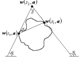
s₀,a ). [image:4.595.236.376.367.466.2]

Although eq. (10) defines a unique invariant for the points in the model, there exist alternative ways in which the points can be chosen. Here we use the geometry shown in figure 1. In this case, the third point is defined by the intersection of the tangents to two points in the curve. The advantage of this definition is that it characterizes a point by only one other point in the image and this point does not require to have a particular geometric relationship to the other two. The definition of the third point is based on the pole-polar form of the shape and it has been previously used for the extraction of circles and ellipses [12]. In [13,14] this relationship is exploited to define indexed tables suited to invariant extraction of shapes by the GHT. These tables store the position of the center of a shape as a function of the invariant properties in the pole-polar form.

Fig. 1. Arrangements of points defined by a pole-polar relationship.

5.3

Local matching

According to eq. (5), we need to solve for the point that satisfies the relationship

(λ0,λ1)=

sim

Q Qsim(υ( ) ( )s0,υ s1). The form of each invariance in this relationship can be obtained by simplifying eq. (10) by using the pole-polar relationships. Thus, invariant features for the points in the model and for the points in the image can be expressed as a function of the position of the points and their gradient direction. The invariance defined in eq. (10) defines two features in the arrangement shown in Fig. 1(b): (1) as a measure of the angle α, between the line joining s0 and s1, and the tangent at s1; and

(2) as a measure of the angle β defined by the intersection of the lines. For the first case we have

( ) ( ) (_{( ) (} )₎ ( ( ) ( )) ( ( )_{( ( )}) (_{) (} )₎

1 0 0

1 0 0 1

0 sim 1 0 0

1 0 0 1

0 sim

s , s s G 1

s , s s G s s Q , s , s G 1

s , s G

, Q

ϕ υ

ϕ υ υ

υ γ

λ γ λ λ

λ

+ − =

+ −

= ,

(11)

for

(

)

(

) (

)

0 1 1 1 1

0,s y y x x

s λ λ λ λ

γ = − − and φ

(

s0, s1

)

=

(

υy

( )

s1 −υy

( )

s0

)

(

υx

( ) ( )

s1 −υx s0

)

. For the

( ) ( ) ( )_{( ) ( )} ( ( ) ( )) ( ( )_{( ( )}) _{) ( )}(₍( ))₎ 1 0 1 0 1 0 sim 1 0 1 0 1 0 sim s G s G 1 s G s G s s Q , G G 1 G G , Q υ υ υ υ υ υ λ λ λ λ λ

λ ′ = ₊ −

+ − =

′ ,, (12)

From eq. (5) we observe that the problem of obtaining a definition of W( )λ0 can be formulated as the problem of obtaining the points υ( )s0 such that the invariant features Qsim(λ0,λ1) and Qsim′ (λ0,λ1) computed from an image are equal to the invariant features Qsim(υ( ) ( )s0 ,υ s1) and Q′sim(υ( ) ( )s0 ,υs1) in the model. That is, for two points in an image, we have a pair of equations that define a pair of points in the model with the same invariant characterization. More formally,

(

0 1

) ( ) ( )

{

0 1 sim

(

0 1

)

sim

(

( ) ( )

0 1

) (

sim 0 1

)

sim

(

( ) ( )

0 1

)}

sim , s , s Q , Q s , s ,Q , Q s , s

W λ λ =υ υ λλ = υ υ ′ λ λ = ′ υ υ (13)

The pair of simultaneous equations can be written as,

( ) ( ( ( )) ( ))( ( ( )) ( )) ( 0 1) ( ( ( )0) ( ( )1))( ( ( )0 ) ( )( 1))

1 0 0 1 0 0 1 0 1 , , 1 , , s G s G s G s G Q s s s G s s s G Q sim sim υ υ υ υ λ λ φ υ φ υ λ λ + − = ′ + − = (14)

The solution of these pair of equations defines the points in eq. (5).

5.4

Parameters of the transformation

A shape’s rotation and scale can be obtained by matching two points of the curve to two points in the model. That is, for each pair of points λ0,λ1∈I, and each pair of points υ( )s0 and υ( )s1 such that Qsim(λ0,λ1)= Qsim

(

υ

( )

sj,υ( )s1

)

and Qsim′ (λ0,λ1)=

( )

( )

(

s , s1

)

Qsim′ υ j υ , we can define a function of the form of eq. (6) as, ( ) ( )

( 0, 1 s0 , s1 )

{

l, Qsim( 0, 1) Qsim(f(( ) ( )l, , s0 ) ( ) ( ),f(l, , s1 ))} f∆ λ λ ,υ υ = ρ λ λ = ρ υ ρ υ (15) By using the geometric properties of a pair of points, it is possible to obtain an explicit form of eq. (15) as,

( ) ( )

( ) ( ) ( ) ( )1 0 0 1 0 x 1 x 0 y 1 y 1 x x y y 1 s s l s s s s tan tan 0 1 0 1 υ υ λ λ υ υ υ υ λ λ λ λ

ρ = ₋−

    − − −     − −

= − − _{, (16)}

6

Affine transformations

6.1

Parametric model

A parametric model for an affine transformation can be obtained by multiplying a model shape υ( )s by a linear transformation. Thus, the parametric model

( a)=

bλ0, λ0−w(s0,a) can be defined by the transformation parameters a=(A,B,C,D)

for the orthogonal components of the parametric model in eq. (9) defined as,

( )s, A ( )s B ( )s w ( )s, C ( )s D ( )s

wx a = υx + υy y a = υx + υy . (17)

6.2

Geometric invariance

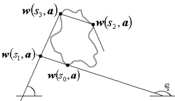
The family of shapes defined by affine transformations is a linear combination of point coordinates. Thus, geometric relationships based on properties computed on a pair of parallel straight lines, such as slope and distance ratio, remain invariant. The distance ratio between two parallel lines can be defined by four points, thus an invariant characterization of a point w

( )

s0,a in the parametric model can be obtained by considering three additional points. If the two points w

( )

s0,a and w

( )

s1,a define a

parallel line to the line formed by the points w

( )

s2,a and w

( )

s3,a , then the distance

ratio invariant for a point w

( )

s0,a can be defined as,

[image:6.595.209.388.114.218.2]

Fig. 2. Arrangement of points to define two parallel lines.

Fig. 2 shows a geometric arrangement that defines invariant features in a manner analogous to Fig. 1. In this case, only three points are on the shape, whilst the fourth one is determined indirectly by using gradient direction information. In this case, the point w

( )

s₁,a is defined by the intersection of the tangent lines to the points w

( )

s₀,a and w

( )

s₃,a .

6.3

Local matching

According to eq. (5), the collection of points W( )λ0 is given by finding the points

( )s0

υ that satisfy the relationship Qaff(λ0,λ2,λ3)= Qaff(υ( ) ( ) ( )s0 ,υ s2 ,υ s3). If we consider the geometry in figure 2, thus this relationship can be written as

( ) ( ( ) ( ) ( )) ( )_{( )} ( )_{( )} 2 x 3 x 0 x 1 x 3 2 0 aff x x x x 3 2 0 aff s s s s s , s , s Q , , , Q 2 3 0 1 υ − υ υ − υ = υ υ υ λ − λ λ − λ = λ λ λ (19) where ( ) ( ) ( ) ( ) ( ) ( )

(

)

( ) ( ) ( ) ( )3 0

y 0 y 3 x x 0 3 y 0 3 x 0 x 3 y y x G G G G G G G G G G 3 0 0 3 1 0 3 3 0 1 λ + λ λ λ − λ λ + λ − λ λ λ = λ λ + λ λ λ + λ λ + λ − λ = λ , (20)

and where υ( )s1 is defined in a similar fashion. By considering the second part of eq. (18), we obtain the invariance definition

( ) ( ( ) ( ) ( )) _{( )}( ) ( )_{( )} 2 y 3 y 0 y 1 y 3 2 0 aff y y y y 3 2 0 aff s s s s s , s , s Q , , , Q 2 3 0 1 υ υ υ υ υ υ υ λ λ λ λ λ λ λ − − = ′ − − =

′ . (21)

Thus, W( )λ0 is given by all the points in the model such that the invariant features

(λ0,λ2,λ3) aff

Q and Qaff′ (λ0,λ2,λ3) computed from an image are equal to the invariant features Qaff(υ( ) ( ) ( )s0 ,υ s2 ,υ s3) and Q′aff(υ( ) ( ) ( )s0 ,υ s2 ,υ s3) on the model shape. That is,

( ) ( ) ( ) ( )

{

( ) ( ) ( ) ( )

( 0 2 3) (aff 0 2 3) aff( ( ) ( ) ( )0 2 3)

}

aff 3 2 0 aff 3 2 0 3 2 0 aff s , s , s Q , , Q , s , s , s Q , , Q s , s , s , , W υ υ υ ′ = λ λ λ ′ υ υ υ = λ λ λ υ υ υ = λ λ λ (22)

This equation and the geometry of the distance ratio define a system of three simultaneous equations. That is,

( )

(

)

( ( ) ( )) ( ) ( )

( )

(

)

(

( ) ( )

)

( ) ( )

( )

( ) ( )( ( )) ( ) ( ) 0. , 0 , , , 0 , , 2 3 2 3 0 0 1 2 3 3 2 0 0 1 2 3 3 2 0 = + − − = + − − = + − − s s s s s G s s s s Q s s s s Q y y x x y y y y aff x x x x aff υ υ υ υ υ υ υ υ υ λ λ λ υ υ υ υ λ λ λ (23)

6.4

Parameters of the transformation

The matching of three points in the curve to three points in the model is sufficient to obtain the parameters A,B,C,D of the transformation. The solution of the parameters of the transformation is defined by the function in eq. (6), and can be developed in a manner analogous to eq. (15). In this case, the parameters are obtained by a system of four equations that define a gathering process in a 4D parameter space. However, the parameter space can be reduced by using the information of the shape's position. After the location parameters have been obtained, we can define two independent systems of two equations. As such, the gathering process can be performed in two 2D accumulators by solving for,

( ) ( )

( ) ( )_{( )} ( )_{( )} ( )_{( )} ( )_{( )}

2 y 2 x 0 y 2 y 2 x 0 x

0 y 0 x 0 y 0 y 0 x 0 x 2 0 2 0

s D s C b s

B s A a

s D s C b s

B s A a s

, s , , f

2 2

0 0

υ υ

λ υ υ

λ

υ υ

λ υ

υ λ

υ υ λ λ

+ =

− +

= −

+ =

− +

= −

∆ _{: (24)}

7

Implementation and examples

To locate a model shape under a similarity transformation, we substitute the definitions in eqs. (13) and (15) into eqs. (7) and (8). Thus, evidence is gathered by using a pair of independent 2D accumulator spaces. The evidence gathering implementation is divided into four steps: (1) for each point λ0in the image chose another point λ1 and compute

(λ0,λ1) sim

Q and Qsim′ (λ0,λ1) according to eqs. (11) and (12); (2) use these values in eq. (14) to find all the points υ( )s0 and υ( )s1 that satisfy eq. (13); (3) use the points λ0,

1

λ , υ( )s0 and υ( )s1 in eq. (16) to find the parameters of the transformation and increment the associated element in the accumulator space; (4) compute the location parameter according to eq. (7). In this implementation, it is important to ensure that both points belong to the same primitive. Thus, the point λ1 is only selected if it is within a specified distance of λ0. In our implementation, λ1 must be closer than one quarter of the image length. We develop the curve υ( )s as an orthogonal Fourier expansion [8]. In this representation, derivatives are easily computed. The system in eq. (14) is solved by using a successive approximation method.

[image:7.595.128.483.556.699.2]

Fig. 3 shows an example of the accumulation process for similarity transformations. This figure contains a synthetic shape with random noise. In this example, 65% of the data corresponds to noise. Fig. 3(b) shows the result of the extraction process superimposed on the original image. Fig. 3(c) and 3(d) show that the location and parameters accumulators contain well-defined peaks.

[image:8.595.144.453.184.407.2]

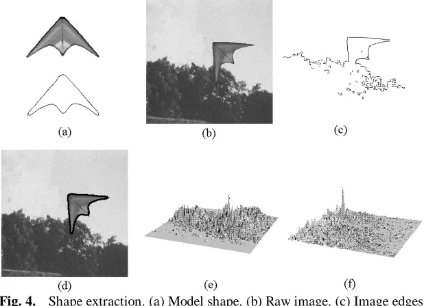
Fig. 4 shows an example of the accumulation process on a real image. The model shape in Fig. 4(a) was obtained from a binary image of 128×128 pixels. The result of the extraction process is presented in Fig. 4(d) superimposed as a thick border. Fig. 4(e) and 4(f) show the final accumulator for the position and for the rotation and scale parameters.

Fig. 4. Shape extraction. (a) Model shape. (b) Raw image. (c) Image edges. (d). Result. (e) Location accumulator. (f) Scale and rotation accumulator. In order to develop an evidence gathering process for affine transformations, we substitute the definitions in eqs. (22) and (24) into eqs. (7) and (8). The evidence gathering process is divided into 5 steps: (1) for each point λ0 in the image choose a pair of points λ2 and λ3 such that the line which passes through the points has the same slope than the gradient direction at the point λ0. From these, compute the value of Qaff(λ0,λ2,λ3) and Qaff′ (λ0,λ2,λ3) according to eqs. (19) and (21); (2) use these values in the system of equations in (23) to find all the points υ( )s0 , υ( )s2 and υ( )s3 ; (3) use the points λ0, λ2, λ3, υ( )s0 , υ( )s2 and υ( )s3 to solve for the parameters

D C B

A, , , ; (4) compute the location parameter according to eq. (6) and increment the associated element in the corresponding position in the accumulator space; (5) after all evidence has been gathered and the location parameter is known, repeat step (1) and use the points in the system of equations in (24) to gather evidence for the parameters of the transformation.

[image:9.595.140.459.114.308.2]

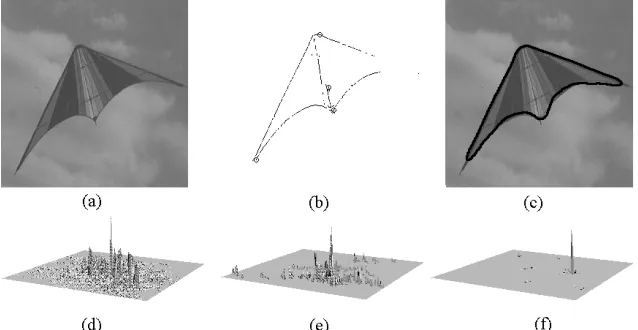
Fig. 5. (a) Model shape. (b) Synthetic image where 35% of the data belongs to the primitive. (c) Result of the extraction process. (d) Location accumulator. (e) Result for

the parameters A and C. (f) Result for the parameters B and D.

[image:9.595.140.459.500.665.2]

Fig. 5 shows an example of the evidence gathered for affine transformations. Fig. 5(a) shows the model shape. Points of high curvature are defined as the zeroes of the derivative of the tangent angle of the Fourier expansion and they are marked with small circles. To quantify which percentage of points is necessary to obtain evidence to locate the shape, we generated a collection of synthetic images containing random noise. The number of points that form the model shape was reduced in proportion to the amount of noise points added to the image. In our experiments we maintained 3 points of high curvature in correct positions (those which lie on the shape), whilst the other five were positioned at random. In the example in Fig. 5, the model shape is composed of 35% of the points (i.e., 65% outliers). Fig. 5(c) shows the result obtained by the gathering process. The accumulator presented corresponds to the parameters of the transformation. An example of the extraction process applied to a real image is presented in Fig. 6.

Fig. 6. Shape extraction. (a) Raw image. (b) Image edges and high curvature points. (c) Result. (d) Location accumulator. (e) Accumulator for the parameters A and C.

8

Conclusions

We have developed a technique for including invariance in a general form of the HT for parametric models defined by similarity and affine transformations. The advantage of this characterization is that it significantly reduces the uncertainty associated with the use of higher level primitives such as lines or curves. Based on invariance characterization it is possible to locate of a shape using a 2D accumulator space. However, the complexity of determining corresponding arrangements of points in the model and in the shape is directly related to the generality of the transformation. We have included an effective strategy that reduces the number of correspondences between the model and the image. This is indispensable since the generality of the transformation increases the geometric complexity of the features identified in the shape. We have shown that the technique can obtain adequate results when some features are generated by background objects or are missed.

References

[1] R.T. Chin, C.R. Dyer, “Model-based recognition in robot vision”, ACM Computing Surveys 18:67-108 (1986).

[2] G. Stockman, “Object recognition and localization via pose clustering”, CVGIP,

40:361-387 (1987).

[3] Y. Lamdan, J Schawatz, H. Wolfon, “Object recognition by affine invariant matching”, Proc. IEEE Conf. on CVPR, pp. 335-344 (1988).

[4] S. Umeyama, “Parameterised point pattern matching and its application to recognition of object families”, IEEE Trans PAMI 15(1):136-144 (1993)

[5] A.Califano, R. Mohan, “Multidimensional indexing for recognition of visual shapes”, IEEE Trans. PAMI 16:373-392 (1994).

[6] D.H. Ballard, D. Sabbah, “Viewer independent shape recognition”, IEEE Trans. PAMI 6:653-659 (1983).

[7] W.E.L. Grimson, D.P. Huttenglocher, "On the sensitivity of the Hough transform for object recognition", IEEE Trans. PAMI 12:255-274 (1990).

[8] A.S. Aguado, M.S. Nixon and M.E. Montiel, Parameterizing Arbitrary Shapes via Fourier Descriptors for Evidence-Gathering Detection, Computer Vision and Image Understanding 69(2): 202-221 (1998).

[9] G. Roth, M. D. Levine, Extracting geometric primitives”, CVGIP: Image Understanding 58:1-22 (1993).

[10]F. Bookstein, “Fitting conic sections to scattered data”, Computer Graphics and Image Processing 9:56-91 (1979).

[11]D. Forsyth, J.L. Mundy, A. Zisserman. C.M. Brown, “Projectively invariant representations using implicit algebraic curves”, Lecture Notes in Computer Science 427:427-436 (1990).

[12]H.K. Yuen, J. Illingworth, J. Kittler, “Detecting partially occluded ellipses using the Hough transform”, Image and Vision Computing 7(1):31-37 (1989).

[13]P.-K. Ser, W.-C. Siu, “A new generalized Hough transform for the detection of irregular objects”, Journal of Visual Communication and Image Representation

6(3):256-264 (1995).