Ac electrokinetics: a review of forces
in microelectrode structures
A Ramos†, H Morgan‡, N G Green‡and A Castellanos†
†Departamento de Electronica y Electromagnetismo, Universidad de Sevilla, Avenida Reina Mercedes, s/n 41012 Sevilla, Spain
‡Bioelectronics Research Centre, Department of Electronics and Electrical Engineering, Rankine Building, Oakfield Avenue, University of Glasgow, Glasgow G12 8LT, Scotland, UK
Received 5 January 1998
Abstract. Ac electrokinetics is concerned with the study of the movement and behaviour of particles in suspension when they are subjected to ac electrical fields. The development of new microfabricated electrode structures has meant that particles down to the size of macromolecules have been manipulated, but on this scale forces other than electrokinetic affect particles behaviour. The high electrical fields, which are required to produce sufficient force to move a particle, result in heat dissipation in the medium. This in turn produces thermal gradients, which may give rise to fluid motion through buoyancy, and electrothermal forces. In this paper, the frequency dependency and magnitude of electrothermally induced fluid flow are discussed. A new type of fluid flow is identified for low frequencies (up to 500 kHz). Our preliminary observations indicate that it has its origin in the action of a tangential electrical field on the diffuse double layer of the microfabricated electrodes. The effects of Brownian motion, diffusion and the buoyancy force are discussed in the context of the controlled manipulation of sub-micrometre particles. The orders of magnitude of the various forces experienced by a sub-micrometre latex particle in a model electrode structure are calculated. The results are compared with experiment and the relative influence of each type of force on the overall behaviour of particles is described.
1. Introduction
The potential for using ac electrokinetic techniques to manipulate and separate bioparticles is now undoubtedly proven. The rapid development of this field into a new technology has been achieved through the application of microelectronic methods used to fabricate small electrode structures that can generate high electrical fields from relatively small applied ac potentials.
The controlled manipulation of cells and micro-organisms has been a topic of research for a number of years. Pohl [1] showed how the application of non-uniform ac fields could induce movement of polarizable particles and termed the force responsible the dielectrophoretic force. It was shown that dielectrophoresis (DEP) could be used to manipulate particles and also to separate different types of bacteria [1]. Recent work has shown the versatility of DEP in areas such as the separation of cancer cells from blood [2] and the separation of bacteria using conductivity or permittivity gradients as a means of controlling the dielectrophoretic forces [3]. A recent review of the subject is given in [4]. The time-averaged DEP force is given by [1, 5]
h ¯FDEPi = 1 2vα∇ ¯E
2
rms (1)
where α is the effective polarizability of the particle,
v is the volume of the particle and ∇ ¯E2
rms is the gradient of the energy density of the electrical field. In order to move particles of the order of 1–10 µm in diameter, a field of 104–105 V m−1 is required.
Early studies of DEP effects were undertaken using large electrode structures (for example a coaxial wire suspended in a tube) and high voltages [1]. However, the application of new micro-fabrication methods has meant that the dielectrophoretic manipulation of particles can be performed using lithographically manufactured micro-electrodes with sufficient field generated using commercially available low-voltage (up to 10 V) frequency synthesizers.
Recent work [6–11] has demonstrated that DEP can be used to manipulate particles smaller than 1µm in diameter. It was believed that the effect of Brownian motion was such that the deterministic movement of such small particles could not be achieved using DEP. The force on a particle due to Brownian motion increases as the particle’s volume is reduced and Pohl [1] showed that excessively large electrical field gradients would be required to move a particle of, for example, 500 nm diameter. However, through the use of electrode structures of a suitable size the electrical field gradient can be increased to a level sufficient
(a)
[image:2.612.317.524.48.268.2](b)
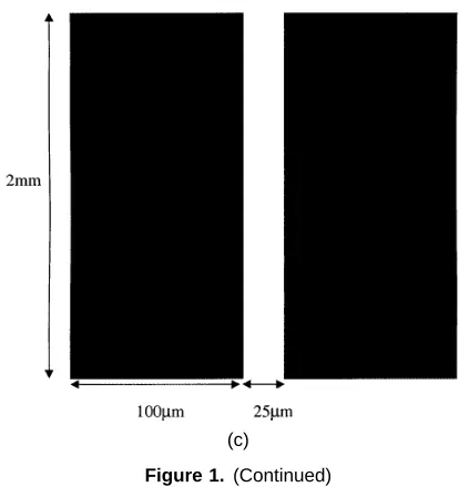
Figure 1. Diagrams of the electrode geometries used in this work. The polynomial electrode is shown in (a) and the castellated one in (b). Dimensions are typically from 2µm to tens of micrometres. (c) Shows a parallel finger electrode used for observation of EHD movement of latex spheres. In this case the electrodes are 2 mm long and 100µm wide, with a 25µm gap.
to move particles of most sizes and types, as recent work has shown. Particles such as plant and animal viruses, latex beads, DNA and macromolecules can be moved by DEP [6–10]. We have also shown that it is possible to
(c)
Figure 1. (Continued)
separate heterogeneous populations of latex particles into sub-populations [11].
Although polarizable particles can be moved using non-uniform electrical fields, the dielectrophoretic force is not the sole force acting on a particle. The total force on any particle is given by the sum of many forces including sedimentation, Brownian, dielectrophoretic and hydrodynamic forces; the latter arising from viscous drag on the particle. An electrical field can also induce fluid motion that will drag the particle and the motive forces are electrohydrodynamic in origin, namely electro-osmosis and electrothermal. The magnitudes of these forces can be of the same order as, or in certain circumstances much larger than, the force exerted on the particle by dielectrophoresis. For example, the movement of particles in micro-electrode arrays is strongly influenced by fluid motion and we [10] together with other workers in the field [6] have noted this fact. At certain combinations of frequency, medium conductivity and applied voltage, the hydrodynamic forces can dominate over the DEP force. Under other experimental conditions these forces are too small to be seen and as a result quite subtle changes in the DEP properties of the particles can be detected and measured [10, 11]. Although these different forces have been observed and noted in the literature, little work has been done to categorize and determine the ranges of sizes of forces and their influences on particles.
[image:2.612.68.281.49.585.2](a)
(b)
[image:3.612.131.467.66.660.2](c)
2. Experimental details
2.1. Electrodes
Electrodes for manipulation and trapping of particles were fabricated using either photolithography or electron beam lithography. Electrodes of the polynomial and castellated geometries were used, details of the design of which have been published elsewhere [10–13]. The polynomial electrode is shown schematically in figure 1(a) and the castellated electrode in figure 1(b). In addition, simple electrodes consisting of two parallel fingers were fabricated, as shown in figure 1(c).
For large particles, such as cells and micro-organisms, electrodes with a spacing of 50–100 µm have been used by other workers. However, the dielectrophoretic manipulation of sub-micrometre latex spheres was performed using inter-electrode spacings in the range 2–25 µm for all of the three electrode designs. Electrodes were manufactured on glass microscope slides with an array covering an area of typically 10 mm×10 mm. Fluorescently loaded latex spheres were obtained from Molecular Probes, Inc and were suspended in a buffer of an appropriate conductivity. The spheres were pipetted onto the electrode array and covered with a glass cover slip. Particle motion was observed with a Nikon Microphot fluorescence microscope and data were recorded with a colour CCD camera and S-VHS video followed by analysis on computer.
2.2. Electrical field calculations
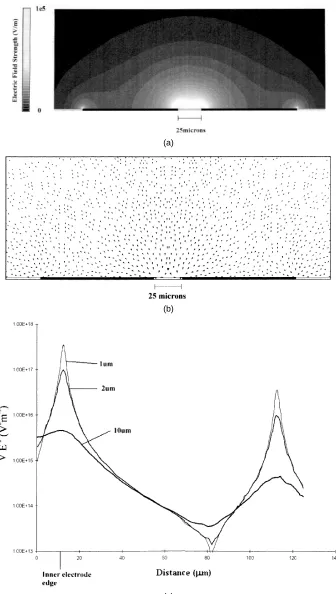
Commercial finite element software (Ansoftr, Maxwell 3-D) was used to generate plots of the electrical field distribution in the electrodes and details of the software have been published elsewhere [10]. Electrical field plots for the polynomial and castellated arrays have been published previously [9–12]. A two-dimensional plot of the field distribution across the parallel finger electrode of figure 1(c) is shown in figure 2(a) at an applied potential of 10 V peak to peak. Figure 2(b) is a vector plot of∇ ¯E2,
which indicates the magnitude and direction of the DEP force on a particle. The sizes of the vectors are drawn on a logarithmic scale. Also shown, in figure 2(c), is a plot of the magnitude of ∇ ¯E2 in a line parallel to the
surface at three different heights (corresponding to 1, 2 and 10 µm). In figure 2(c) the mid-point between the two electrodes is at 0 µm and the electrode edge is at
+12.5µm. It is clear from these figures that a minimum in electrical field and force exists at a point equidistant between the two fingers, with a secondary minimum on top of the electrodes. The maximum in field strength is at the edge of the electrodes and particles would be expected to collect here under positive DEP.
2.3. Experimental observations
[image:4.612.317.533.55.312.2]It has been shown that sub-micrometre latex spheres exhibit a frequency-dependent dielectrophoretic force [10, 11]. At high frequencies the particles are less polarizable than the medium and experience negative dielectrophoresis. At low
Figure 3. Fluorescence photographs of 282 nm latex particles undergoing dielectrophoresis in micro-electrode arrays. The inter-electrode gap was 4µm and the medium conductivity was 11 mS m−1. (a) Shows spheres collecting under positive DEP at the tips of castellated electrodes. The frequency of the applied field was 1 MHz and the applied voltage was 10 V peak to peak. In this photograph the electrodes appear brighter than the surround. At high frequencies, 10 MHz, the spheres undergo negative DEP and are trapped in a triangle formation in the bays, as shown in (b). In (b) the electrode array is illuminated from beneath so that the electrodes appear dark.
frequencies the particle is always more polarizable than the medium and undergoes positive DEP. The transition from positive to negative DEP is characterized by the frequency at which the polarizability of the particle is
zero. For 282 nm spheres suspended in a 1 mM
potassium phosphate buffer (σm = 18.5 mS m−1) this occurs at a frequency of approximately 5 MHz [10], with a relaxation corresponding to the Maxwell–Wagner interfacial polarization of the bead and the medium. At lower frequencies the polarizability of a latex bead increases due to the presence of the ionic double layer, resulting in an increase in the dielectrophoretic force on the particle. For the 282 nm spheres the effect of the double layer in the DEP spectrum becomes apparent for higher medium conductivities and for 10 mM potassium phosphate buffer (σm=0.17 S m−1) the cross over from negative to positive DEP occurs at a frequency in the range 70–200 kHz [10].
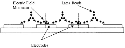
Figure 4. A photograph showing the pattern of spheres collecting on top of the electrodes as a result of
hydrodynamic effects. At a frequency below 0.1 MHz the 282 nm spheres collect as diamond-shaped aggregates on top of the electrodes. This photograph was taken at an applied potential of 10 V peak to peak. In this photograph the electrodes are lighter than the background.
in agreement with literature results for larger particles such as cells and micro-organisms [4, 14]. At high frequencies the spheres experience negative DEP and collect in the bays between the electrode tips, as shown in figure 3(b). Figure 3(b) was taken at an applied frequency of 10 MHz, 10 V peak to peak. This image was taken with the electrodes back illuminated to increase the contrast, so that the electrodes appear black in the photograph, whereas in figure 3(a) the electrodes are lighter than the background. At frequencies below 200 kHz, the spheres remain at the electrode tips under positive DEP but also experience a force moving them into the central region of the electrode. The magnitude of this force increases both with increasing field strength and with decreasing frequency. At a sufficiently low frequency (<0.1 MHz) and at a suitable field strength all the spheres can be collected in the central region of the electrode, as shown in figure 4. This figure shows diamond-shaped aggregates of spheres sitting on top of the electrodes. The effect is reversible: increasing the frequency of the applied voltage results in spheres moving back to the electrode tips. This has been observed for a range of sizes of spheres from 93 to 557 nm diameter, for which the trend is the same but the voltage and frequency at which the effect occurs are different for each size of bead. The larger particles require a larger applied voltage or a lower frequency to move them into the centre. The flow of particles into this region is observed to be from the electrode edge into the centre of the electrode. These observations are general for a range of electrode geometries and particle sizes. Other workers [15] have made similar observations of the movement of yeast cells into the central region of a castellated electrode array. We have repeated these experimental observations both with live yeast and with latex particles and find the trends to be the same. The effects are inconsistent with the predicted movement of particles solely by DEP.
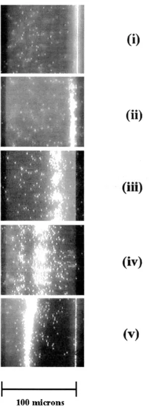
[image:5.612.64.286.51.229.2]Figure 5 shows a sequence of photographs of 282 nm spheres on top of a parallel finger electrode of the design shown in figure 1(c) taken as a function of the frequency. For clarity only one half of the array is shown. The inter-electrode gap was 25µm and the suspending medium was KCl of conductivity σm = 2 mS m−1. The photograph of figure 5(i) clearly shows the spheres being attracted to the electrode edge under positive DEP at a frequency of 90 kHz and voltage of 10 V peak to peak. The remaining sequence shows the effect of decreasing the frequency. At a frequency of 60 kHz, fluid flow occurs, causing particles to move away from the edge of the electrode into an equilibrium position on top of the electrodes. In figure 5(ii) this equilibrium represents a balance between positive DEP forces attracting particles to the electrode edge and a drag force exerted on the particle by field-induced fluid movement moving into the electrode centre. The sequence (iii)–(v) is a time sequence showing how the spheres move in towards a point which is the minimum in electrical field at a distance two thirds of the way in from the inter-electrode gap (see also the field plot of figure 2(b)). Figures 5(iii) and (v) show that, at a potential of 10 V peak to peak and a frequency of 5 kHz, the spheres form two lines either side of the field minimum as particles are driven by fluid flow from both edges of the electrodes. These two lines eventually merge into one continuous ribbon as shown in figure 5(v). This photograph was taken at an applied potential of 16 V peak to peak and a frequency of 5 kHz. The particles form a continuous band at the electrical potential minimum, but also some particles are attracted by positive DEP to the electrode edge. This sequence of photographs illustrates that the movement of particles onto the top of an electrode is not a dielectrophoretic effect as had been reported in the literature.
3. Force calculations
For the remainder of this paper we will estimate the order of magnitude of the force on sub-micrometre solid latex particles of 282 nm diameter in an electrode consisting of two parallel fingers separated by a 25 µm gap, as shown in figure 1(c). The particles are suspended in a 500 µm KCl solution of conductivity 8 mS m−1. When appropriate, the predicted and experimentally measured forces are compared.
3.1. Dielectrophoresis
For a homogeneous dielectric particle suspended in an aqueous medium the dielectrophoretic force given by equation (1) can be rewritten in the form [5]
¯
FDEP = 12Re[(m¯(ω)·∇)E¯∗] (2)
where E¯∗ is the complex conjugate of the electrical field and m¯(ω) is the dipole moment which, for a spherical particle, can be expressed as
¯
m(ω)=4π εma3K(ω)E¯ (3)
withωthe angular field frequency,athe particle radius and
K(ω)the Clausius–Mossotti factor given by
K(ω)= ε˜p− ˜εm ˜ εp+2ε˜m
(4)
where ε˜p and ε˜m are the complex permittivities of the particle and the medium respectively. For an isotropic homogeneous dielectric, the complex permittivity is
˜
ε=ε−jσ
ω (5)
where j = √−1, ε is the permittivity and σ is the conductivity of the dielectric. For realE¯, the time-average DEP force is found by substituting equation (3) into (2) and is
h ¯FDEP(t )i =2π εma3Re[K(ω)]∇| ¯Erms|2 (6)
where∇| ¯Erms|2 is the gradient of the square of the RMS
electrical field. The absolute value of the force on a particle depends on ∇| ¯Erms|2 and also on the real part of K(ω), the in-phase component of the particle’s effective polarizability. For a sphere the real part ofK(ω)is bounded by the limits 1 < Re[K(ω)] < −12 and varies with the frequency of the applied field and the complex permittivity of the medium. Positive DEP occurs when Re[K(ω)]>0, the force is towards points of high electrical field and the particles collect at the electrode edges. The converse of this is negative DEP which occurs when Re[K(ω)]< 0, the force is in the direction of decreasing field strength and the particles are repelled from the electrode edges.
For small particles (<1 µm diameter) it can be seen from equation (6) that large electrical field gradients are required to produce the forces required to induce motion. The use of micro-fabricated electrodes to generate high fields has meant that the dielectrophoretic movement of sub-micrometre particles has been established beyond doubt. However, observations of the movement of sub-micrometre particles in planar micro-electrode arrays as a function of the frequency and applied voltage have not been undertaken in any detail. On this scale the dielectrophoretic force can be of the same order as other forces acting on the particle and it is important to be able to distinguish each force. These forces can be generally classed into those which act indirectly on the particle through viscous drag due to fluid movement, namely electrohydrodynamic (EHD) forces, and those acting directly on the particle, such as sedimentation and Brownian motion.
3.1.1. The DEP force. Given knowledge of the frequency-dependent dielectric properties of the particle and medium (the Clausius–Mossotti factor) and the electrical field gradient, an order-of-magnitude estimate of the DEP force can be made for a range of particle sizes from equation (6). At an applied potential of 10 V peak to peak and at a point 10 µm in from the edge of the electrode and heights of 1, 2 and 10 µm the magnitudes of the field gradient were calculated using finite element methods, see figure 2(c). Estimating the gradient to be of the order
|∇E2
the limiting low-frequency DEP force (for the Maxwell– Wagner interfacial relaxation) can be calculated asFDEP = 10−14 N. Using Stokes’ law, this gives a particle velocity
of vDEP = FDEP/(6π ηa) = 5 µm s−1, where η is the viscosity of the suspending medium. As figure 2(c) shows, the field gradient increases rapidly towards the electrode edge (by up to two orders of magnitude) and the particle velocity will increase to as much as 500µm s−1.
3.2. EHD forces
3.2.1. Electrothermal forces. The high electrical fields used to manipulate small particles imply that there is a large power density generated in the fluid surrounding the electrode. The power generation per unit volume is given by
W =σ E2(W m−3). (7)
The order of magnitude of the total power generated can be calculated for the parallel electrodes shown in figure 1(c) as follows. Taking a typical medium conductivity of
σm = 0.01 S m−1 and an average electrical field of 4 × 10⁵ V m−1 (corresponding to an applied voltage
of 10 V in a gap of 25 µm), then the average power dissipation in the inter-electrode volume can be calculated to be 1.6×10⁹W m−3. The volume over which this heat
is generated is typically very small and for the parallel finger electrodes shown in figure 1(c) can be estimated to be approximately 50 µm×50 µm×2 mm (long) = 5×10⁻¹²m3, giving an average power dissipation of 8 mW.
This value can be compared with the power dissipation measured for the electrode. The measured resistance,R, of this electrode array in the same medium was 33 k and, with an applied potential of 20 V peak to peak, the total power dissipation is V2
rms/R = 1.5 mW. In general, for micro-electrode structures of these typical dimensions and at this conductivity, the power dissipation will be of the order of 10 mW.
The generation of this amount of power in a very small volume could conceivably give rise to a large temperature increase in the sample. In order to estimate the temperature rise for a given electrode array the following energy balance equation must be solved [16]:
ρmcpv¯·∇T +ρmcp
∂T ∂t =k∇
2T +σ E2 (8)
where v is the velocity, T the temperature, ρm the mass density, cp the specific heat (at constant pressure), k the thermal conductivity and σ the electrical conductivity of the medium.
The typical diffusion time for the temperature front can be estimated from the thermal conductivity or Fourier equation [16]:
∂T ∂t =
k ρmcp
∇2T . (9)
An order of magnitude analysis of this equation gives the time,tdiff, as
tdiff =
ρmcpl2
k (10)
where l is the characteristic length of a system. For water, k = 0.6 J m−1 s−1 K−1 and c
p = 4.18 × 10³ J kg−1 K−1 so that, for l = 20 µm (a typical
inter-electrode distance), tdiff ≈ 10−3 s, implying that thermal equilibrium is established within 1 ms of applying the electrical field. In an ac field the total temperature, T, can be written asT =T0+1T (t ), whereT0 is the time-average temperature and1T (t )depends on 2ω (twice the frequency of the applied field). Thus from equation (9) the differential temperature 1T /T ≈1/(2ωtdiff)and, for fields of frequency greater than 1 kHz, the differential temperature change is negligible, namely1T /T 1.
In a micro-electrode array under steady-state condi-tions, the effect of fluid motion on the temperature profile,
∇T, in equation (8) is assumed to be minimal. For this to be true
|ρmcpv¯·∇T| |k∇2T| (11) which from dimensional analysis of equation (8)
ρmcpvl
k 1. (12)
Experimental observation of the movement of particles, such as latex spheres, in micro-electrode structures at higher frequencies shows that the velocity of the particles is in the range 1–10 µm s−1. Assuming that the fluid velocity is
of the same order of magnitude, then, with l = 20 µm,
ρmcpvl/ k ≈10−2 1 so that the effect of fluid flow on the temperature profile can be neglected even for a fluid velocity approaching 1 mm s−1. Thus fluid flow does
not influence the temperature field and for a planar micro-electrode system under steady-state conditions (t >1 ms) equation (8) can be simplified to
k∇2T+σ E2=0. (13)
An order-of-magnitude estimate of the incremental temperature rise can be made by substituting for the electrical field in equation (13) to give
k1T l2 ≈
σ V2
rms
l2
or
1T ≈ σ V 2
rms
k (14)
whereVrmsis the potential difference across the electrodes. In this case the electrodes are assumed to be perfect heat sinks (with the electrical and temperature gradients changing over the same length scale). For an applied potential V = 20 V (peak to peak) and with σm = 0.01 S m−1, the temperature rise can be calculated to be
1T ≈1◦C. (Detailed analysis of a parallel plate geometry has been performed and the calculations give a smaller temperature rise, see appendix A.)
covered with a glass microscope cover slip. For a solution of conductivity 0.07 S m−1 and withV = 20 V peak to
peak the measured steady-state temperature rise was 2◦C, compared with a calculated rise of 6◦C; for a conductivity of 0.008 S m−1the rise was 0.2◦C compared with a
calcu-lated value of 0.7◦C. The data were measured over a broad range of applied frequencies from 1 kHz to 20 MHz and the temperature change was found to be the same for all frequencies, in accord with equation (14).
Equation (14) also shows that, for high-conductivity solutions, the temperature rise is likely to be excessive and for biological systems could lead to denaturation of the material. For example, using 100 mM phosphate buffer, with σm=1 S m−1, the temperature rise would approach 100◦C for the same applied voltage, but this would depend on the geometry of the system. This is in quantitative agreement with more detailed calculations on temperature gradients in capillary electrophoresis systems [17].
Reducing the dimensions of the system will lower the voltage required to produce a given electrical field strength and as a result reduce both the power dissipated in the system and the temperature increment (see equation (14)). Therefore, micro-electrode technology is the obvious means to achieve low-temperature dielectrophoresis, particularly for the DEP movement of sub-micrometre particles.
Since the electrical field is highly non-uniform the power density is also highly non-uniform. A variation in the temperature of a liquid such as water causes local changes in the density, viscosity, permittivity and conductivity of the medium and these inhomogeneities will give rise to forces on the fluid. The most common is the buoyancy force, which arises when a temperature gradient produces changes in the density of a liquid giving rise to natural convection. The other force is electro-thermal and arises from the fact that changes in conductivity and/or permittivity with temperature give rise to gradients in the medium. The conductivity gradient produces free volume charge and the Coulomb force whilst a permittivity gradient produces the dielectric force.
3.2.2. Coulomb and dielectric forces. A general expression for the electrical force per unit volume on a liquid is [18]
¯
fE=ρqE¯ − 1 2E¯
2∇ε+1
2∇
ρm
∂ε ∂ρm
¯
E2
(15)
where ρq is the volume charge density and ε is the permittivity of the medium. For an incompressible fluid the last term in this equation has no effect on the dynamics (it is the gradient of a scalar) and therefore will be ignored in the subsequent analysis [18]. For an isothermal fluid there is no free charge and the permittivity gradient is zero so that the total force is zero. Localized Joule heating gives rise to gradients in permittivity and conductivity, which in turn cause an electrical force causing fluid motion. For small temperature rises the gradients in permittivity and conductivity can be written as ∇ε = (∂ε/∂T )∇T and ∇σ = (∂σ/∂T )∇T respectively, so that an order-of-magnitude estimate of these forces can be made as
follows. Assuming that the deviations of the permittivity and conductivity are small, the electrical field can be written as the sum of two components, the applied field, E¯0,
and the perturbation field, E¯1, where E¯ = ¯E0+ ¯E1 and |E1| |E0|. An expression for this force can be obtained, to a first-order approximation, by rearranging equation (15). Given that ρq = ∇·(εE¯), substituting for the total field givesρq = ∇ε·E¯0+ε∇·E¯1, where we have taken into
account that ∇·E¯0 =0. WithfE¯ =ρqE¯0−12E¯02∇ε and
substituting for the free charge we can write
¯
fE=(∇ε·E¯0+ε∇·E¯1)E¯0−12E¯02∇ε. (16)
The charge-conservation equation is∇·(σE¯ +ρqv¯)+
∂ρq/∂t =0, whereρqv¯ is the convection of charge. This equation can be simplified, since in our case the divergence of the convection of charge is negligible compared with the divergence of the ohmic current
|∇·(ρqv¯)|
|∇·(σE¯)| ' ρqv¯
|σE¯| =
|∇·(εE¯)v¯|
|σE¯| '
ε/σ l/v 1
where l and v are the typical distance and velocity, respectively. The ratio of the convective and ohmic currents is of the order of the ratio of the charge relaxation time of the liquid and the typical time taken to travel the distance
l. Taking a typical distance of 20 µm and a maximum velocity of 200 µm s−1 we get a time of 0.1 s, which
is several orders of magnitude greater than typical charge relaxation times in aqueous solutions.
Substituting for E¯ in the charge-conservation equa-tion and neglecting the convective term, we have
∇σ·E¯0+σ∇·E¯1+ ∂
∂t(∇ε·E¯0+ ∇ε·E¯1)=0. (17)
If the electrical field is time varying, namely E¯0(t ) =
Re(E¯0ejωt)then the conservation of charge is
∇σ·E¯0+jω∇ε·E¯0+σ∇·E¯1+jωε∇·E¯1=0. (18)
Rearranging this equation gives the divergence of the perturbation field:
∇·E¯1=
−(∇σ+jω∇ε)·E¯0
σ+jωε (19)
assuming that the liquid is non-dispersive in the frequency range of interest.
The time-averaged force per unit volume is then†
hfEi = 12Re[(∇ε·E¯0+ε∇·E¯1)E¯0∗−12|E0|
2∇ε] (20)
and substituting for the divergence of the perturbation field gives
hfEi = 1 2Re
(σ∇ε−ε∇σ )·E¯0 σ+jωε
¯
E0∗−1 2|E0|
2∇ε
.
(21)
Figure 6. A diagram showing an electrode arrangement used for the analytical model, equation (24), for the temperature field. It consists of two parallel plates with a very small inter-electrode gap. The plates are covered in a dielectric (water) and a potential ofV (in volts) is applied across the gap. The direction of the field is shown.
In our case E¯0 is real and equation (21) can be simplified
to
hfEi = −1 2 ∇σ σ − ∇ε ε
·E¯0 εE¯0
1+(ωτ )2 +
1 2|E0|
2∇ε
(22) where τ = ε/σ is the charge relaxation time of the liquid. The first term on the right-hand side of the equation represents the Coulomb force and the second term the dielectric force.
In certain frequency ranges either the Coulomb force or the dielectric forces dominate. The transition from dominance by one force to dominance by the other occurs at a frequency at which the magnitude of the Coulomb force becomes equal to the magnitude of the dielectric force. From equation (22) this frequency,fc, is given by
ωc =2πfc≈ 1 τ 2 ∂σ σ ∂T ∂ε ε∂T 1 2 . (23)
For water (1/σ )(∂σ/∂T ) = +2% per degree and
(1/ε)(∂ε/∂T ) = −0.4% per degree [19] so that the magnitude of the square root in equation (23) is approximately 3. The cross over frequency, fc, is then of the order of the inverse of the charge relaxation time of the liquid given by τc≈τ =ε/σ.
An order-of-magnitude estimate of the force on the liquid can be made for a simple analytical system. Consider two thin parallel metal plates, with a very small inter-electrode gap mounted on an insulator with liquid above the plates. The plates are subjected to a potential difference,V
that sets up an electrical fieldE¯(r, θ )as shown in figure 6. Neglecting end effects, an analytical expression for the electrical field is given by [20]
¯
E(r)=V π
1
rnˆθ (24)
and the power dissipated per unit volume is
W (r)=σ E2=σ V 2
π2
1
r2.
Substituting for this explicit expression for power in the temperature balance equation (13) gives
k r ∂ ∂r r∂T ∂r + k r2
∂2T ∂θ2 = −
σ V2 π2
1
r2. (25)
A particular solution to this equation is
Tp= −
σ V2θ2
2π2k .
Assuming that the electrodes behave as thermal baths, the boundary conditions at θ = 0 and θ = π are T = 0 (the reference temperature is chosen to be zero). The boundary conditions at the electrodes together with the particular solution of equation (25) lead to solutions of T
that are functions of θ only and independent of the radial co-ordinate r. Then, the solution for the temperature of equation (25) that also satisfies the boundary conditions at
θ =0 andθ =πis simply
T (θ )= −σ V 2θ2
2π2k + σ V2θ
2π k (26)
with
Tmax=T
π
2
= σ V2
8k .
For the time-averaged ac case the temperature field depends on the RMS voltage. The gradient of temperature is
∇T = σ V2
2π k
1−2θ
π
1
rnˆθ. (27)
Given the temperature field, the force on the liquid can be computed exactly from equation (15). Substituting for the temperature gradient into equation (22), where
∇σ =(∂σ/∂T )∇T and∇ε=(∂ε/∂T )∇T, then the time-averaged force with an applied alternating potential is
hfEi = −M(ω, T )
εσ V4
rms
2kπ3r3T 1−
2θ π
ˆ
nθ (28)
where
M(ω, T )=
T σ ∂σ ∂T − T ε ∂ε ∂T 1+(ωτ )2 +
1 2 T ε ∂ε ∂T (29)
is a dimensionless factor which gives the variation of the force as a function of the frequency. A plot of the magnitude ofMagainst frequency atT =300 K is shown in figure 7. It can be seen that M is positive for low frequencies and negative for high frequencies, with the cross over frequency approximately equal tofc. The force on the fluid depends on the angle,θ, with the maximum at
θ =0 orπ. The force per unit volume can be calculated and, for σm = 0.01 S m−1, V = 10 V (peak to peak),
r = 20 µm and T = 300 K, then| ¯fE|/M =12 N m−3, which in the low-frequency limit gives a maximum force of | ¯fE| ≈ 80 N m−3. For low frequencies the force is
Figure 7. A plot of the magnitude of the factorM(ω,T)
(see the text), as a function of the frequency.
Figure 8. A diagram showing the motion of fluid at frequencies below the charge relaxation time of the liquid (given by equation (23)) for the electrode geometry of figure 6. Fluid moves down into the inter-electrode gap and out across the electrode. The direction of the arrows would be reversed at high frequencies above the charge
relaxation time.
The velocity field,v¯, of the fluid can be obtained from the Navier–Stokes equation that, for low Reynolds number, is written [16]
η∇2v¯− ∇p+ ¯f=0 (30)
together with the mass-conservation equation, which for an incompressible fluid is
∇·v¯ =0 (31)
where η is the viscosity, p the pressure and f¯ a general volumetric force. For flow in micro-electrode structures the Reynolds number, Re, is very small and can be calculated from Re = ρmvl/η, where l is again the characteristic length. From our observations of the velocity of a range of sub-micrometre latex spheres the maximum velocity was
vmax ≈200µm s−1and, withl=10µm,Re=2×10⁻³ 1 so that equation (30) is applicable.
In our case the velocity can be obtained by solving equations (30) and (31), with the appropriate boundary conditions and with the expression for the electrical force. The case of a local solution is detailed in appendix B. To a first approximation, the velocity can be obtained by comparing the viscous force component with the
electrothermal force, fE¯ to get vf luid ≈ | ¯fE|l2/η. Again using a characteristic length ofl=20µm, the flow velocity can be calculated to be in the rangev≈4–40µm s−1in the high- and low-frequency limits respectively. The detailed analysis outlined in appendix B shows that the velocity is smaller by a factor of 0.13 than this simple calculation shows, ranging from 0.7 to 5 µm s−1 at r = 20 µm
with 10 V (peak to peak). It is instructive to compare the fluid velocity with typical velocities for sub-micrometre particles in a DEP force field. As an example, for a 282 nm latex bead we can use equations (6) and (24) to estimate the force on the particle in the planar electrode geometry shown in figure 6. For this structure the electrical field gradient can be written as ∇E2 = −[2V2/(π2r3)]nˆ
r, so that the DEP force at r = 20 µm with V = 10 V peak to peak is FDEP = 4×10⁻¹⁵ N (assuming that the real part of the Clausius–Mossotti factor is+1). Using Stokes’ equation, the particle velocity is vDEP =1.8 µm s−1. It can be seen that this is of the same order of magnitude as the fluid flow, particularly for frequencies belowfcand therefore electrothermally induced fluid flow could have marked effects on the observations of the DEP force for this size of particle.
An explicit expression relating the magnitudes of the DEP and electrothermal velocity for any particle of radius
a, in an electrode of a geometry shown in figure 6, with applied potentialV can be derived from equations (6) and (28):
vf luid
vDEP
=0.13 3 4π
M(ω, T )
Re[K(ω)]
σ V2
rms
kT r2
a2 (32)
where the numerical factor (0.13) accounts for the geometry of the particular system shown in figure 6, see appendix B. This equation can be rearranged to give the proportionality between the fluid and DEP velocities:
vf luid
vDEP
∝σ V2r 2
a2 (33)
which shows that fluid flow increases directly with the medium conductivity. Also this equation shows that the DEP force dominates close to the electrode edges (as expected) and that the influence of fluid flow gets progressively bigger for smaller particles.
For polynomial electrode arrays, it has been observed [6, 21] that fluid flow causes particles to be trapped in the centre of the electrode by a combination of DEP forces and hydrodynamic forces. This effect takes place at high frequencies at which the particles undergo negative DEP and the fluid-flow pattern is dominated by the permittivity term. At high frequencies the force on the fluid is given by h ¯fEi → −1
4| ¯E0|
2∇ε. Muller et al
[image:10.612.62.286.266.362.2]and E¯2 only. As a consequence fluid will flow from
regions of high permittivity (low temperature) to regions of low permittivity (high temperature), which can be seen as movement from outside the electrode along the inter-electrode regions (where the field is maximum) and up and out through the central part.
In our experimental observations we have noted anomalous fluid movement at low frequencies which cannot be explained by this theory. These effects will be discussed in section 3.2.4.
3.2.3. Natural convection. A temperature gradient gives rise to a change in fluid density and thus natural convection is to be expected. The magnitude of this effect can be estimated by comparing the electrothermal force and the buoyancy force.
The buoyancy force is given by
¯
fg=1ρmg¯=
∂ρm
∂T 1Tg¯ (34)
whereg¯ is the acceleration due to gravity. Substituting for the temperature rise from equation (26), the buoyancy force is
¯
fg=
−σ V2θ2
2π2k + σ V2θ
2π k
∂ρm
∂T g¯. (35)
The maximum temperature rise and force occur when
θ = π/2, so that Tmax = T (π/2) = σ V2/(8k). For the same parameters as those used above, namely σm = 0.01 S m−1 and V = 10 V (peak to peak), with (1/ρm)(∂ρm/∂T )=10−4 per degree andg =9.81 m s−2, then |fg| = 0.026 N m−3. It is clear that this value is considerably smaller than the value calculated for the volume force due to the electrothermal effect. Even for a characteristic length of 100 µm the electrothermal force is in the range 0.1–0.7 N m−3 which is still much bigger than the buoyancy force. Again dimensional analysis over a characteristic length of l=20µm gives
1ρmg¯
1 2E
2∇ε
≈1ρmg¯l
1 2E
2ε
1
and thus, for all situations involving micro-electrode structures, the effects of natural convection are negligible compared with those of the electrical forces.
[image:11.612.316.532.51.134.2]3.2.4. Other EHD forces. Both literature data [15] and our observations of the low-frequency behaviour of biological particles in non-uniform ac electrical fields show that the motion of the particles does not follow that expected for conventional dielectrophoresis. For example it has been reported [15] that yeast cells form diamond-shaped aggregates on top of the electrode in castellated micro-electrode arrays; patterns were observed for frequencies below 500 Hz. This was interpreted as low-frequency negative DEP coupled with electrophoretic effects acting on the cells. We have observed similar patterns using latex spheres across a wide range of sizes, applied frequencies and medium conductivities. For example figure 3(a) shows a pattern of latex spheres experiencing positive DEP
Figure 9. A diagrammatic representation of the motion of 282 nm diameter latex particles and, by implication, of fluid flow for applied frequencies of 50 kHz and below. Spheres move from the bulk liquid into the inter-electrode gap and then out across the electrode surface, finally collecting in the centre.
collecting on the electrode tips. At lower frequencies the spheres also formed patterns on top of the electrodes, as shown in figure 4. For frequencies above 5 MHz the spheres experience only negative DEP and collect as small triangles in the electrode bays where the field gradient is minimum (figure 3(b)), in accord with other observations on cells and micro-organisms [4, 15]. Although the diamond patterns on top of the electrode have been interpreted as dielectrophoretic in origin [15], our observations lead us to believe that the patterns are caused by fluid movement. The collection of particles on top of the electrodes occurs below a threshold frequency. Increasing the applied field increases the collection rate. In all cases the aggregations were observed for a range of particle types and sizes from 93 nm to 10 µm in diameter, but the effect occurred at different threshold frequencies for each particle size. Using 25µm gap finger electrodes and 93 nm spheres in a medium of conductivity 8 mS m−1 the threshold frequency was
0.5 MHz, but for yeast cells in 8 mS m−1buffer the effect
occurred at frequencies below 1 kHz. This leads us to believe that fluid flow, rather than DEP, dominates the effect.
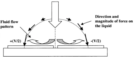
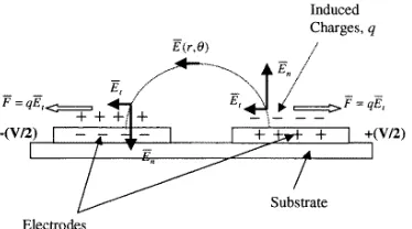
Figure 10. An outline of the electrostatic situation on a parallel plate electrode array showing how the radial field can be resolved into normal and tangential components. The tangential component of the field gives rise to a Coulomb force on the fluid, namely electro-osmosis, which causes fluid to move out across the electrode from the edge to the centre.
This flow pattern is similar to that expected from electrical forces induced by Joule heating of the liquid (see section 3.2.1 above) at frequencies below the cross over frequency, fc, given by equation (23). However, we have noted that the velocity of the flow pattern increases with decreasing frequency and also with increasing applied voltage, approximately proportional to V2. It has been
shown above that electrothermal effects are independent of frequency, except around fc. Also for electrothermal effects the fluid velocity is proportional toV4, rather than
toV2. Since EHD forces cannot be invoked to explain the flow patterns, we are led to believe that the origin of this force is other than electrothermal. We will consider the influence of the electrical double layer on fluid flow, in a process analogous to electro-osmotic fluid flow under a dc potential.
For a parallel planar micro-electrode configuration a schematic representation of the electrical field configuration close to and above the electrodes is shown in figure 10. Application of a voltage to the electrode causes charge to appear at the electrode–electrolyte interface, which changes the charge density in the electrical double layer as shown in figure 10. The time for the establishment of this charge distribution is of the order of the charge relaxation time,
τ [22]. If the applied potential is alternating then, for any frequency below f = 1/(2π τ ), the charge on the electrode and in the double layer will alternate in each half cycle of the applied potential. In the case of dc electro-osmosis, this charge will experience a force tangential to the electrode surface, given by F = QEt, where Et is the tangential electrical field and Q is the charge in the double layer. This force will act on the double layer and cause fluid movement, which we call ac electro-osmosis by analogy with dc electro-osmosis. As shown in figure 10, the direction of the force on the charge and thus the fluid-flow pattern are independent of the sign of the applied voltage since the sign of the excess charge in the double layer is always opposite to that of the charge on the electrode. Both the sign ofQand that ofEtchange with each half cycle, so that the direction of the forceFis constant. The magnitude of the forceF is obviously a function of the magnitudes of
QandEt and will vary from a maximum at the electrode
edge, where bothQ andEt are maximum, to a minimum near the centre of the electrode, whereEt is zero.
For dc electro-osmosis, the fluid velocity, v, in the double layer is given by [17]
v= Etσq
κη (36)
whereσqis the surface charge density andκ−1is the Debye length of the diffuse double layer. This equation assumes a tangential electrical field with a magnitude that is invariant along the length of the double layer and a surface charge defined as
σq=
Z ∞
0 ρqdz
whereρq is the volume charge density in the double layer andzis the direction normal to the surface. This equation may not be completely applicable in our case since both
ρq andEt are functions of distance in all directions. For micro-electrode structures with strongly divergent fields the tangential field will vary with distance, both normal to the surface and along the surface. At a distance corresponding to the Debye length,Etis much smaller thanEn; however, it is of sufficient magnitude to induce a large tangential force which could result in fluid motion. An estimate of the electrical field for the electrode structure shown in figure 10 has been made using finite-element field analysis software. With an inter-electrode gap of 25 µm and an applied voltage of 10 V peak to peak, then at a distance of 10 nm from the surface (a typical Debye length) and 10µm in from the electrode edge,En=3.4×10⁴ V m−1 and Et = 50 V m−1. Although this tangential field is much lower than that used in dc electro-osmosis, the surface charge density is much higher in this case. For a Debye length of 10 nm, the average specific capacitance of the double layer can be estimated to be of the order of 0.1 F m−2(fromC=ε
mκ). The voltage across the double layer varies with the applied frequency; at low frequencies almost the entire applied voltage will be dropped across the double layer whereas at high frequencies the potential drop across the double layer goes to zero due to polarization of the electrode/solution interface [23, 24]. Assuming that the double-layer voltage is 10% of that across the solution then the average double-layer charge density, σq, can be estimated to be 50 mC m−2(for an applied voltage of 10 V peak to peak). From equation (36) this translates into a time-averaged fluid velocity of 21µm s−1. (If the distance
is reduced to 2 µm, then Et is ten times bigger and the fluid velocity increases to 200µm s−1.)
3.3. Brownian motion and diffusion
Forces other than electrical and gravitational also act to move particles. The principal non-deterministic force acting on an ensemble of sub-micrometre particles is that due to diffusion. Diffusion driven by Brownian motion was generally regarded as a ‘disrupting’ force in that it was considered that the dielectrophoretic movement of sub-micrometre particles could not be achieved at realizable field strengths [1]. However, recent experimental work has shown that the DEP force required to induce movement of sub-micrometre scale particles is in the sub-picoNewton range. For example, the force required to initiate observable movement of a tobacco mosaic virus (a 300 nm×18 nm diameter rod) can be estimated from measurements to be of the order of 10−15 N [25]. Our measurements
of the velocity of a Herpes simplex virus (a 250 nm diameter spherical particle) in a micro-electrode array gives a slightly larger force, in the range (1–2) × 10−14 N.
These forces are much lower than the force required to move a particle estimated from the simplistic diffusion argument of Pohl [1]. These forces can be easily generated using a simple point–point electrode configuration with an electrical field of the order of 106 V m−1. The movement
of macromolecules using dielectrophoresis has also been reported [8], showing that, even for such small objects, the randomizing effect of Brownian motion is not significant enough to hinder DEP collection.
Brownian motion is a stochastic process, so the time-averaged movement of a particle undergoing Brownian motion is zero. Irregular motion of the molecules in the liquid imparts random forces on a particle in suspension. The collisions are irregular and over time the distribution of the random displacement of the particles follows a Gaussian profile with a mean squared displacement (in one dimension) given by [26]
|1x¯|2=2Dt (37)
whereDis the diffusion coefficient. For a spherical particle of radiusa, this is given by
D= kBT
6π ηa (38)
wherekB is the Boltzmann constant.
The equation of motion of an isolated colloidal particle can be written as the sum of three components, the acceleration force, the friction force (equal to 6π ηav¯ for a spherical particle) and the randomizing force. On balancing these forces one obtains the Langevin equation [27]:
mdv¯
dt = −fv¯+ ¯Fr(t ) (39)
wheremis the particle’s mass,f is the friction factor and
¯
Fr(t ) is the randomizing force due to Brownian motion. The solution of this equation gives a Gaussian probability distribution of the particle having a velocity v at timet. For very short times the individual particle displacements depend on t and the motion is uniform. For longer time intervals the displacement depends on √t and is given by equation (37), whereD=kT /f.
The transition from a directional to a random process (from a process which varies withtto one which varies with
√
t) depends on the mass of the particle and the viscosity of the medium. The time of this transition is given by [28, 29]
t0=m/f. For a colloidal particle of diameter 100 nm the time is O(10−8) s. This means that the energy imparted to a particle by a thermal impulse decays on a time scale
t0 =m/f. Clearly, observations of thermal velocities are difficult, the time of observation being less thant0.
In terms of the dielectrophoretic movement of a particle, it is important to note that the time-averaged randomizing force due to Brownian motion is zero; that is,h ¯Fr(t )i =0. The problem of defining a threshold force for DEP movement of particles then becomes a matter of solving the Langevin equation to assign the probability of a particle being found at a certain point after a given time. An alternative way of viewing this process is to consider the probability distribution of the position of a single particle in an isolated system. Application of a uniform force will perturb the probability distribution so that the centre of the Gaussian profile will move in the direction of the force field. Defining the centre of the Gaussian to be x¯, then in the presence of a deterministic force and after a short time there will be a displacement fromx¯ tox¯+1x¯. After time1t this is given by
1x¯ = F¯
6π ηa1t. (40)
The probability of finding a particle around the new position of x¯ +1x¯ has a Gaussian distribution that is bounded by equation (37). The particle has uncertainty in its position given by this Gaussian profile. We can define an
observable deterministic force to be a force which produces
a displacement which is greater than the uncertainty in the position, namely|1x¯|>3(2Dt )1/2 corresponding to three standard deviations from the mean position. Using this equality, then, for a 282 nm diameter bead and over an observation time of 1 s, a force of 1.4×10⁻¹⁴N will cause
an observable deterministic movement. The force required is smaller with √t, so that over 10 s the force required is 4.7×10⁻¹⁵ N. These forces are of the same order of magnitude as those measured experimentally. The longer the time frame of observation the smaller the force required to produce an observable movement. For example with the application of a force 104times smaller, the necessary time
of observation increases to 3 years!
Obviously these calculations are applicable only to the movement of a single isolated particle and could be used to calculate the movement of isolated particles in micro-electrode structures. For a collection of particles a statistical approach must be used to predict the movement and distribution of the ensemble [30]. The particle-conservation equation is then
∂n
∂t + ¯v·∇n= −∇·JT¯ (41)
where n is the number of particle per unit volume and
¯
J is the total flux consisting of the sum of the diffusion, sedimentation and DEP fluxes, namely
¯
with
¯
JD= −D∇n Jg¯ = nFg¯
6π ηa JDEP¯ = nFDEP¯
6π ηa
where the gravitational and DEP forces have been defined previously.
A classic example of this is the balance of sedimentation and diffusion for particles in solution. Ignoring electrostatic particle–particle interaction, the gravitational force acts downwards, pulling particles out of the solution phase. The resulting increase in concentration of particles at the bottom of a vessel creates a diffusion force acting upwards [31]. The system either reaches a steady state with particles suspended in the bulk in a distribution related to the forces on the particles or complete sedimentation takes place when diffusion is negligible compared with gravity.
The case of the dielectrophoretic collection of particles on a plane is similar except that the DEP force must be added to the gravitational force. For a suspension of particles, when the DEP force is first applied the equilibrium is disturbed. If the DEP force is strong enough to hold the particles at an electrode surface, there is an immediate decrease in the concentration of the particles above the electrodes. This induces a local concentration gradient above the electrodes so that a diffusion flux acts in the same direction as DEP, pushing particles towards the electrodes. This will occur indefinitely as long as particles are entirely removed from the solution phase (an infinite sink). Therefore, in large devices the dielectrophoretic collection and concentration of sub-micrometre particles could be as efficient as for cells and micro-organisms because the diffusion force is greater and acts in concert with the DEP force. If the DEP force is weak and particles are not immobilized at the surface (for example in pearl chains) then redistribution of the bulk concentration will occur until the system reaches a steady state and the net flux is zero in a manner analogous to sedimentation.
The particle-conservation equation can be used to analyse the confinement of particles in potential energy minima such as for a particle held under negative DEP in a polynomial electrode array [13]. In this case particles are confined within a circle whose radius represents the balance between electrical and thermal energies. Within this radius the particle is free to move since its thermal energy is always greater than the dielectrophoretic potential energy. Beyond the boundary the DEP energy is greater than the particle’s thermal energy and the particle remains confined in the trap. From the diffusion equation, in the steady state the total flux at any point is zero. In this case the particle-conservation equation can be written as
−D∇n+nF¯DEP
6π ηa =0. (43)
By solving the first-order differential equation for
n we obtain the Boltzmann expression in terms of the dielectrophoretic potential energy, UDEP =
−2π εma3Re[K(ω)]| ¯Erms|2, as
n=n0exp
−
UDEP
kT
. (43)
On substituting the explicit expression for the DEP energy with K(ω)= −0.5, then for a 282 nm diameter bead the DEP potential energy is equal and opposite to the thermal energy,kT, whenE=2.6×10⁴V m−1. In order to confine
99% of the particles inside this radius then
exp
−
UDEP
kT
=0.01
and the field must be increased toE =5.6×10⁴ V m−1. Preliminary observations confirm the order of magnitude of these calculations.
4. Conclusion
Order-of-magnitude calculations for the force on sub-micrometre particles in non-uniform ac electrical fields have been computed. It has been shown that, for low-conductivity solutions, the effect of Joule heating on the total temperature of the system can be neglected. For example with a medium conductivity of 0.01 S m−1 and a maximum applied potential of 20 V peak to peak the overall temperature rise in a micro-electrode system will be only of the order of 1◦C, a value confirmed by experiment. For sub-micrometre particles the electrothermal effects have been shown to be of sufficient magnitude to compete with DEP forces. For example, both Coulomb forces and dielectric forces give rise to fluid motion. At a certain cross over frequency fc, these two forces are equal in magnitude, but for frequencies belowfc, the Coulomb force dominates, whereas for frequencies above this the dielectric force is dominant. This cross over frequency is of the order of three times the charge relaxation frequency of the liquid and for a solution of conductivity 0.01 S m−1 is
approximately 7 MHz. For parallel finger electrodes an analytical expression for the electrical field was used to compute the range of fluid velocities. For a conductivity of 0.01 S m−1and an applied voltage of 10 V peak to peak this
ranged from 0.7µm s−1(at high frequencies) to 5µm s−1at frequencies below fc. This compares with a typical DEP-induced particle velocity of 1.8 µm s−1 for the 282 nm
diameter particles at the same distance from the electrode edge. The DEP-induced velocity varies much more rapidly with the distance to the electrode edge than does the electrothermally induced fluid velocity (equation (32)), and can reach 200µm s−1 near the electrode edge, compared
with a fluid velocity of the order of 50µm s−1. In
micro-electrode structures, if there are thermal effects induced by Joule heating, natural convection is very small compared with the electrothermal forces and therefore this effect can be neglected.
Over a range of frequencies, voltages and conductivi-ties, typically below 500 kHz for a medium conductivity of up to 0.1 S m−1, an additional driving force acting on the
fluid can be identified. The fluid motion moves particles away from the electrode edge and into well defined regions
on top of the electrodes. In this case the fluid velocities
Brownian motion has been shown to be less of an impediment to the dielectrophoretic movement of nano-scale particles than was considered by other authors. For example, the observable deterministic force required to move a particle of 282 nm diameter can be calculated to be of the order 2.4×10⁻¹⁴ N over a 1 s time frame of
observation, compared with an experimental value of the order of (1–2)×10−14 N for a Herpes simplex virus of 250 nm diameter. Diffusion can also act in concert with DEP forces to increase the rate at which a DEP system collects sub-micrometre particles. For a particle confined in a potential energy minimum, a comparison between the DEP potential energy and the thermal energy can be used to estimate the magnitude of the potential energy required to confine a particle within a given boundary. In this case the electrical field can be estimated to be of the order of 5×10⁴ V m−1.
In conclusion, although the DEP-induced deterministic movement of sub-micrometre particles can be complicated by hydrodynamic effects, it has been shown that the forces on particles can be predicted and therefore controlled. Consequently it can be foreseen that recent technological advances in dielectrophoresis could be applied, together with electrohydrodynamic fluid movement, to develop new methods for the characterization, manipulation and separation of sub-micrometre and nano-scale particles.
Acknowledgments
The authors wish to acknowledge the UK Engineering and Physical Sciences Research Council for the award of a studentship to NG Green and for financial support from the British Council and Acciones Integradas programme. We also wish to acknowledge the UK Biotechnology and Biological Sciences Research Council (grant 17/T05315) and the Spanish Direcci´on General de Ense˜nanza Superior (research project PB96-1375).
Appendix A
Heating in a parallel plate capacitor
Taking a planar capacitor with separation d between the plates, the equation to solve is
kdT
dx2 = −σ E
2 (A1)
with boundary conditionsT =T0at the plates (x=0 and
x=d). The solution is
T =T0+σ E 2d
2k
x−x 2
d
. (A2)
The maximum temperature is reached in the centre of the gap between the electrodes and, from (A2), is
T =T0+σ E 2d2
8k . (A3)
The temperature rise is 1T = σ Vrms2 /(8k). For σm = 0.01 S m−1 andV =20 V peak to peak, the temperature
rise can be calculated to be1T =0.1◦C.
Appendix B
In the steady state the equation of motion is
−∇p+η∇2v¯+ ¯fE=0 (B1)
wheref¯Eis given by equation (28) of the text. Taking the curl of this equation and assuming two-dimensional flow, the stream function9 is found from
−η∇49+(∇ × ¯fE)·nzˆ =0 (B2)
where nzˆ is the unit vector in the z direction and the velocity is obtained from the stream function, v¯ = ∇ ×
(9nzˆ ). Taking into account the expression for the force, equation (28) of the text, the following expression (in polar co-ordinates) must be solved:
1 r ∂ ∂r r∂ ∂r + 1 r2 ∂2 ∂θ2 2
9= 2C r4
1−2θ
π
(B3)
where
C=M(ω, T )
εσ V4
rms 2kπ3T η
. (B4)
We assume solutions are of the form 9(r, θ ) = rnf (θ ). The rdependence of the right-hand side of equation (B3) implies that9is a function of the angleθonly. The general solution of equation (B3) that is a function ofθ only is
9= −C
2 θ2 2 − θ3 3π
+A1sin(2θ )+A2cos(2θ )+A3θ+A4 (B5) whereAn are constants defined by boundary conditions.
The boundary condition for zero velocity atθ =0 and
θ =π implies that:
∂9
∂θ =0 atθ=0, π.
Since the stream function is defined except for a constant then, without loss of generality, we have
9=0 forθ =0, π.
The symmetry of the system implies that
∂29
∂θ2 =0 atθ =0, π/2.
Thus the final solution is
9= −C
2 θ2 2 − θ3 3π −Cπ
24[sin(2θ )−2θ]. (B6)
Substituting this into the expression for the stream function, the velocity is
vr= 1 r ∂9 ∂θ = C r −1 2
θ−θ 2
π
− π
12[cos(2θ )−1]
.
(B7) The velocity is radial and the maximum for a given radial distance is
vmax=
π
24
C r
which occurs at θ = π/2. The velocity is zero for