An Improvement in the Artificial-free Technique along the Objective Direction for the Simplex Algorithm

An Improvement in the Artificial-free Technique

along the Objective Direction for the Simplex

Algorithm

Aua-aree Boonperm

Abstract—The artificial-variable free technique along the objective direction for the simplex algorithm was proposed for solving a linear programming problem in 2014. It was designed to deal especially with unrestricted variables. Before starting the simplex algorithm, a single unrestricted variable is rewritten us-ing two nonnegative variables causus-ing the number of variables increasing. In this paper, we present that this technique can deal with nonnegative variables which the real world problems needed the variables to be nonnegative. Moreover, we propose some criteria for selecting a variable to transform the problem. The computational results show that the average number of iterations from the selected variable which has the maximum coefficient of the objective function outperform the original simplex algorithm.

Index Terms—artificial-free, linear programming, trans-formed problem, relaxed problem, objective direction.

I. INTRODUCTION

T

HE simplex algorithm [1] has been popularly used to solve linear programming problems and it is quite efficient in practice for small or medium size [2]. However, in 1972, a collection of linear programming problems which shows the worst case running time for the simplex algorithm using the original Dantzig’s rule was given by Klee and Minty [3]. Then, Karmarkar [4] has proposed a new faster algorithm and many researchers have improved pivoting rule for the simplex algorithm [5]. However, finding the new initial feasible point which is closer the optimal point and solving without artificial variables were proposed [2], [6], [7], [9], [10], [11], [12].

The simplex algorithm starts at an initial basic feasible solution, x=0 (the origin point). If the origin point is not a basic feasible solution then the artificial variables will be added for finding the basic feasible solution. Big-M and Two-Phase method are well-known algorithms which are used to handle artificial variables. By adding artificial variables, the number of variables will be increased.

In 1997, Arsham [6], [7] proposed the algorithm without using artificial variables. However, in 1998, Enge and Huhn [8] proposed a counterexample, in which Arsham’s algorithm declared the infeasibility of a feasible problem.

In 2000, the algorithm for solving a linear programming problem without adding artificial variables was proposed again by Pan [9]. The algorithm starts at the initial basis

Manuscript received January 8, 2017; revised February 2, 2017. This work was supported in part by the Department of Mathematics and Statistics, Faculty of Science and Technology, Thammasat University Rangsit Center, Thailand (sponsor and financial support acknowledgment goes here).

A. Boonperm is with the Department of Mathematics and Statistics, Faculty of Science and Technology, Thammasat University Rangsit Center, Pathum Thani, 12121, Thailand. e-mail:[email protected]

which corresponds to a solution in primal and a solution in dual. If the primal solution and the dual solution are infeasible, then costs of objective function in primal will be perturbed to some positive number for dual feasibility and the dual simplex method can start. The computational results were shown to be superior for small problems and this algorithm starts from the origin point.

Arsham [10], [11] then presented the new solution algo-rithm without using artificial variables repeatedly in 2006. Before the algorithm starts, the right hand side values need to be nonnegative. The simplex algorithm can start without using artificial variable by relaxing the≥ constraints. Then all relaxed constraints will be reinserted to the problem to guarantee the optimal solution. However, the computational result was not shown the effectiveness of the algorithm. In that year, Corley et al. [12] proposed the algorithm without introducing artificial variables for nonnegative right hand side problems. They solve the relaxed problem which consists of the original objective function subject to a single constraint which makes a largest cosine angle with the gradient vector of the objective function. At each subsequent iteration, the constraint which had the new maximum cosine angle among those constraints would be added, and the dual simplex method is applied. However, their research is restricted for a feasible and bounded linear programming problem and the computational experiment was not shown.

is rewritten using two nonnegative variables causing the number of variables increasing by a factor of two for each unrestricted variable.

From the artificial-free techniques above, in this paper, we improve the artificial-free technique along the objective direction [13] by suggestion the criteria to choose the variable which is used to map the problem. Moreover, the improved algorithm can deal with the nonnegative varaiables. The proposed algorithm starts by using the objective plane to split constraints into three groups by considering the sign of coefficient for each constraint. Then constraints from the nonpositive groups (negative and zero coefficient groups) are relaxed. The relaxed problem can identify a feasible point by our theorem. Then it will be transformed for starting the sim-plex algorithm without using artificial variables. Constraints from the nonpositive groups are added for checking the solution from the relaxed problem. Since artificial variables is not used, the number of variables by our algorithm is less than or equal to the number of variables by the simplex algorithm. The number of constraints which solved by our algorithm is less-than or equal to the number of constraints which solved by the simplex algorithm. This is an obvious advantage of our algorithm. Moreover, we suggest the criteria to select the variable for mapping. From the computational results, we found that iterations from the selected variable which has the maximum cost of the objective function outperform the simplex algorithm, and another criteria. The main concept of our algorithm and theorems for guarantee feasibility of a relaxed linear programming problem is shown in section 2. In section 3, after the relaxed problem is solved by the simplex algorithm, constraints from the negative group and the zero group will be added and analysed for finding the optimal solution. In section 4, the computational results show the effectiveness of the algorithm. In the last section, we conclude and discuss our new findings.

II. PRELIMINARIES

Consider a linear programming problem in the following form:

Maximize cT_x

subject to Ax ≤b x ≥0

(1)

where c is a nonzero vector and x is an n-dimensional column vector,Ais anm×nmatrix,bis anm-dimensional column vector. Let

y=cTx=c1x1+c2x2+· · ·+cixi+· · ·+cnxn. (2)

Ifci6= 0, we determine

xi =

y ci

−

n X

j=1

j6=i

cj

ci

xj. (3)

After replacingxi into the problem (1), the problem in an

equivalent form can be written as follows:

Maximize y

subject to ali ciy+

n P

j=1

j6=i

(alj− alicj

ci )xj ≤bl, l= 1,2, ..., m y

ci − n P

j=1

j6=i cj

cixj ≥0

x1, ..., xi−1, xi+1, ..., xn ≥0.

(4)

Sincexi ≥0, _cy

i−

n P

j=1

j6=i cj

cixj ≥0 is added to be the(m+

1)th _{constraint. Then the problem (4) can be rewritten as}

follows:

Maximize y

subject to y ≤b0r− n P

j=1, j6=i

a0_rjxj, r∈M1

y ≥b0_s−

n P

j=1, j6=i

a0_sjxj, s∈M2

n P

j=1, j6=i

atjxj ≤bt, t∈M3

x1, ..., xi−1, xi+1, ..., xn ≥0.

(5) whereM1, M2andM3 are the set of the constraintr, s, t if ari

ci >0, asi

ci <0and ati

ci = 0 respectively, andb

0

l=c_aibl li, a0_lj= cialj

ali −cj,l∈ {M1∪M2},j= 1,2, ..., nandj6=i.

Consider the (m+ 1)th constraint, we let a0_m+1,j = cj,

j= 1, ..., i−1, i+1, ..., nandb0

m+1= 0. Ifci>0thenm+1

will be added toM2. Otherwise,m+ 1will be added toM1. So|M1|=m1,|M2|=m2,|M3|=m3andm1+m2+m3=

m+ 1.

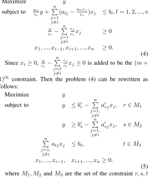
Since we classify groups by the value of coefficients,M1is the group of positive coefficients,M2is the group of negative coefficients, andM3is the group of zero coefficients.

0

optimal point y

x₂ M2

M1

M3

[image:2.595.306.549.73.363.2]

M2

Fig. 1. Example of a feasible region after mapping inR2

Pleasantly, the problem (5) can be written in the matrix form as follows:

Maximize y

subject to 1m₁y ≤b0_m1−A0_m1x¯i, 1m₂y ≥b0_m3−A0_m2x¯i, Am₃x¯i ≤bm3

x¯i ≥0

(6)

where 1m₁ is an m1-dimensional column vector of 1,

1m₂ is an m2-dimensional column vector of 1, b0_m1, b0_m2

andbm₃ are the right hand side vector corresponding to the group M1, M2 andM3, respectively. A0m1, A

0

m2 andAm3

are submatrices corresponding to the groupM1,M2andM3, repectively.x¯Ti = [x1, x2, ..., xi−1, xi+1, ..., xn]

A. The relaxed problem

Consider the problem (6), it will be feasible when y is between constraints in the group of M1 and constraints in groupM2, andx¯_i satisfies constraints in groupM3 as figure 1. Since we want to maximize y, the optimal solution will be formed by some constraints from groupM1. So we will relax some constraints from groupM2andM3. Then, we will solve the problem with constraints from the groupM1 first. Therefore, the relaxed problem can be rewritten as follows:

Maximize y

subject to 1m1y ≤b

0

m1−A

0

m1x¯i x¯_i ≥0

(7)

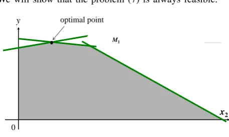
We will show that the problem (7) is always feasible.

0 y

M1 optimal point

[image:3.595.53.282.221.358.2]

x₂

Fig. 2. Example of a feasible region of the relaxed problem (7) inR2

Theorem 1. If M1 6= ∅ and b0min = min r∈M1

{b0_r}. Then

(y0,x¯Ti0) = (b

0

min,0T) is a feasible point of the problem

(7).

Proof:SupposeM16=∅andb0min= min

r∈M1

{b0_r}. Choose (y0,x¯Ti0) = (b

0

min,0 T

). We get 1m1y0 =1m1b

0

min ≤ b

0

m1.

So(y0,x¯Ti0) = (b

0

min,0 T

)is a feasible point of the problem (7). The problem (7) is always feasible.

If M1 = ∅ and M3 = ∅ then the problem (6) can be rewritten as follows:

Maximize y

subject to 1m₂y ≥b0_m2−A0m2x¯i, x¯i ≥0

(8)

We can show that the problem (8) is unbounded.

Theorem 2. If M1 =∅ and M3 =∅ then the problem (8)

is unbounded.

Proof: Assume M1 = ∅ and M3 = ∅. Let X =

{(y,xT

¯

i )|1m2y ≥ bm2 −A

0

m2x¯i} and b

0

max = max s∈M2

{b0_s}. Show that X is not empty.

Choose (y0,x¯_iT₀) =(b0max,0

T_{). We get 1m}

2y0 =

1m2b

0

max ≥ b

0

m2. So (y0,x T

¯_i0) = (b0max,0 T₎

is a feasible point of the problem (8). So X is not empty.

We will show that dT _{= [1,0, ...,0]}T _{is a recession}

direction[1] wheredis ann-dimensional column vector. For all α > 0 and (y0,x¯T_i0) +αdT = (y0+α,x¯T_i0+α0T) = (y0 +α,x¯T_i0) ∈ X. Since 1m2y0 ≥ b

0

m2 −A

0

m2x¯i0 and 1m₂α >0,

1m₂(y0+α) =1m2y0+1m2α≥b

0

m2−A

0

m2(x¯i0+0)

=b0_m

2−A

0

m2x¯i0.

Thereforedis a recession direction ofX.

Consider the objective cost of the problem (8) is cT ₌

[1,0, ...,0]T_,(y

0+α,xT¯_i0+α0T)c=y0+α. Sinceα >0,

y0 +α → ∞ as α → ∞. Therefore the problem (8) is unbounded.

B. The transformed problem

The relaxed problem (7) is always feasible. If b0_m1 ≥ 0 then (y0,x¯Ti0) = 0

T

is a feasible point and we can start the simplex algorithm by adding slack variables. Otherwise, (y0,x¯Ti0) = (b

0

min,0 T

)is a feasible point. Then we transform the problem (7) using y0 _{=y−y0. The equivalent form is}

in the following:

Maximize y0+y0

subject to 1m₁y0+A0_m1x¯i ≤b0m1−1m1y0 x¯i ≥0

(9)

Constraints of group M2 will be transformed as

1m2y

0_+A

m2x¯i≥b

0

m2−1sy0. The variable y is not in

constraints in groupM3. So constraints in group M3 is not transformed. The transformed problem can be written in the following:

Maximize y0+y0 subject to 1m1y

0_+A0

m1x¯i ≤b

0

m1−1m1y0 1m2y

0_+A0

m2x¯i ≥b

0

m2−1m2y0 Am3x¯i ≤bm3

x¯_i ≥0

(10)

If the transformed problem is infeasible or unbounded then the problem (6) will be infeasible or unbounded, respectively. If the optimal solution of the transformed problem (y0∗,x¯i∗

T

) is found then the optimal solution (y∗,x¯i∗

T

)of the problem (6) will be found by lettingy∗=y0∗+y0. Then optimal so-lution of the original problem is

x∗¯_i

x∗¯_i

=



 

y∗ ci −

n P

j=1

j6=i cj cix

∗

j

x∗¯_i



 .

III. THE PROPOSED ALGORITHM

Consider the problem (9), we found thatb0_m

1−1m1y0≥0.

So the standard form can be written as follows:

Maximize y+_−y−_+y

0

subject to 1m₁y+−1m₁y−+A0_m1x¯i+s =b0m1−1m1y0 y+, y−,x¯i,s ≥0

(11) Letˆbm₁=b0_m1−1m₁y0. So the initial tableau of the relaxed problem (11) can be shown as follows:

z y+ y− x¯i s RHS

z 1 -1 1 0T ₀T _y

0

s 0 1m1 −1m1 A

0

m1 Im1 ˆbm1

A. The optimal solution case

After we found the optimal solution of the problem (11), then we will check that it will be the optimal solution of the original problem by adding constraints from group M2 andM3into the problem (11). For the transformed problem, constraints of groupM2will be changed as1m2y

0_+A0

m2x¯i≥ b0_m

2 −1m2y0 or −1m2y

0_−A0

m2x¯i ≤ −bm2 +1m2y0. The

standard form for the transformed problem is −1m₂y+₊

1m₂y−−Am₂x¯i+sM2 =−bm2 +1m2y0 where sM2 is a

nonnegative column vector. Let Bm∗

1 and Nm∗1 are the optimal basis and the

associ-ated nonbasic matrix of the problem (11), respectively. The corresponding tableau of the relaxed problem is as follows:

z xBm∗₁ xNm∗₁ RHS

z 1 0 ZN_m∗

1 −c

T N_m∗

1 zm∗

1 +y0

xBm∗₁ 0 Im1 B

−1 m∗ 1Nm ∗ 1 B −1 m∗ 1 ˆ bm1

whereZN_m∗

1 ,=cT

B_m∗

1 B−_m1∗

1Nm

∗

1,zm

∗

1=c

T B_m∗

1 B−_m1∗

1

ˆ

bm₁,cT B_m∗

1

and

cT_N

m∗₁ are costs of objective function vectors of the problem

(11) which rearranged by basic and nonbasic columns.

Let Aˆ =

−1m₂ 1m₂ −A0_m2

0 0 Am₃

be the combined

co-efficient matrix of group M2 and M3. I23 =

Im₂ 0 0 Im₃

where Im2 is an m2×m2 identity matrix and Im3 is an

m3×m3 identity matrix. b23 =

−b0_m2−1m₂y0

bm₃

So the

additional constraints from the groupM2andM3is rewritten as follows:

ˆ

AB_m∗

1 xB_m∗

1

+ ˆAN_m∗

1 xN_m∗

1

+I23s23=b23 (12) where Aˆ = [ ˆABm∗₁,AˆNm∗₁] are rearranged by basic and

nonbasic columns. After adding constraints (12) into tableau, we get

z xBm∗₁ xNm∗₁ s23 RHS

z 1 0 ZN_m∗

1

−cT N_m∗

1

0 zm∗

1+y0

xBm∗₁ 0 Im1 B

−1

m∗

1Nm

∗

1 0 B

−1

m∗

1

ˆ

bm₁

s23 0 AˆBm∗₁ AˆNm∗₁ I23 b23

We can eliminateAˆBm∗₁ by multiplying the second row by

ˆ

AB_m∗

1 and subtracting from the third row gives the following

tableau:

z xBm∗₁ xNm∗₁ s23 RHS

z 1 0 ZNm∗₁ −c

T N_m∗

1

0 zm∗

1+y0

x_Bˆ

m∗₁ 0 Im1 B

−1

m∗

1Nm

∗

1 0 B

−1

m∗

1

ˆ

bm₁

s23 0 0 Aˆ

0

Nm∗₁ I23

ˆ

b23

where ˆb23 = b23−AˆBm∗₁B

−1

m∗

1

ˆ

bm1 and Aˆ

0

N_m∗

1

= ˆANm∗₁ −

ˆ

ABm∗₁B

−1

m∗

1Nm

∗

1. We can obtain the optimal solution by

con-sidering the sign of the right hand side in rows23. Ifˆb23≥0, then the current solution is optimal. Otherwise, perform the dual simplex method to find the solution. Then we can conclude that if we find the optimal solution by the dual simplex method using Dantzig’s rule, the value of the right hand side in the optimal tableau is the optimal solution of the

transformed problem. Otherwise, if the dual is unbounded, we can conclude that the original problem is infeasible.

B. The unbounded case

LetBm₁ be the basis andNm₁ be the associated nonbasic matrix of the problem (11). The corresponding tableau of the relaxed problem is as follows:

z xBm1 xNm1 RHS

z 1 0 ZNm1−c

T

Nm1 zm1+y0 xBm₁ 0 Im1 B

−1

m1Nm1 B

−1

m1

ˆ

bm1

where ZNm1 = c T Bm1B

−1

m1Nm1, zm1 = c T Bm1B

−1

m1

ˆ

bm1.

Let R be an index set of nonbasic variables and zj = cT

Bm1B

−1

m1Nm1:j,j∈R. If the relaxed problem is unbounded,

it means that there iszj−cj<0andBm−11Nm1:j≤0. We will

find the solution of the transformed problem by adding all constraints from groupM2 andM3 into the current relaxed tableau.

Similarly, we can use the equation (12) like the optimal solution case for adding to the current tableau when Bm∗

1

andNm∗

1 are replaced byBm1andNm1. After elimination, if

ˆ

b23≥0, then the current solution is primal feasible then the primal simplex will be applied. Otherwise, both primal and dual solutions are infeasible at the current iteration because of zj−cj <0. In [9], his method perturbs zj−cj <0 to

a positive value to obtain the dual feasible and then perform the dual simplex. After the optimal solution is found, the original zj−cj will be restored and the primal simplex is

used. However, if the dual problem is unbound, then the original problem is infeasible.

C. The special case

IfM1=∅ andM2=∅ then the problem (6) remains in the following

Maximize y

subject to Am3x¯i ≤bm3 x¯_i ≥0

(13)

From the problem (13), the solution can be one of two cases: unbounded or infeasible. Because of the variableyis not in constraints, if there is x¯i0 that Am3x¯i0 ≤ bm3 then

the problem is feasible and y can increase to infinity. So the problem will be unbounded. Otherwise, the problem is infeasible. In this case, we will start with the first constraint and relax the remaining constraints as in the following:

Maximize y

subject to aT

1:x¯i ≤b1

x¯i ≥0

(14)

wherea1: is the coefficient vector of the first constraint. For fixing j ∈ {1,2, ..., n}, ifa1j 6= 0 wherej 6=i then

y= 0, xj =_ab_1j1 andxl= 0is a feasible point of the problem

(14) where l = 1,2, ..., n, l6=j 6=i. Then the transformed problem is

Maximize y

subject to a11

aljx1+· · ·+x

0

j+· · ·+ a1n

aljxn+ s= 0 x1, ..., x0j, ..., xn, s≥0

wherex0_j =xj−_ab_1j1. This problem is unbounded. Then we

will add the remaining constraints and use the unbounded case for checking the solution.

D. Summary of the algorithm

The algorithm is summarized in the following:

Step 1: Map the original problem with xi=y−(c1x1+

ci−1xi−1+· · ·+ci+1xi+1+· · ·+cnxn)/ciwhere

ci6= 0to the problem (4) and split constraints into

3 groups.

Step 1.1: If M1 6= ∅, relax constraints from group M2 and M3. If b0

r ≥ 0 for all r ∈ M1, start the

simplex algorithm at the origin point. Other-wise, transform the problem usingy0 =y−b0_min

where b0_min = min

r∈M1

{b0_r} and start the simplex algorithm.

If the optimal solution is found, go to Step 2 (the optimal solution case.). Otherwise, go to Step 3.

Step 1.2: Otherwise, if M3 = ∅, the problem is un-bounded. Then stop.

Otherwise, relax constraints from the groupM3 and transform the problem usingy0 =y−b0max

whereb0max= max s∈M2

{b0s}. This relaxed problem

is unbounded. Go to Step 3 (the unbounded case.).

Step 2: Test the optimal solution with all constraints from groupM2 andM3.

Step 2.1: If it satisfies all constraints, it is the optimal solution. Then stop.

Step 2.2: Otherwise, perform the dual simplex at the unsatisfied constraints until the optimal solution is found. Then stop.

Step 3: Add all constraints from groupM2 andM3. Step 3.1: If the current solution satisfies all constraints,

perform the primal simplex algorithm until the optimal solution is obtained. Then stop. Step 3.2: Otherwise, perturb the negative reduced cost to

a positive value for dual feasibility, then per-form the dual simplex until the optimal solution is found. Restore the original reduced cost and perform the primal simplex until the optimal solution is found. Then stop.

E. The proposed criteria

In this paper, we suggest three criteria to choose the mapping variable as follows:

1. Choose the variable which has the smallestm1. 2. Choose the variable which has the largestm1.

3. Choose the variable which has the largest coefficient of the objective function.

IV. COMPUTATIONALRESULTS

In this section, we tested the algorithm based on simulated linear programming problems. The randomly generated lin-ear programming test problems

- are maximization problems;

- have a vectorcwithci∈[−9,9], i= 1,2, ..., n;

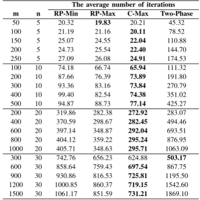
TABLE I

COMPARISON THE AVERAGE NUMBER OF ITERATIONS BETWEEN THREE CRITERIA ANDTWO-PHASE METHOD

The average number of iterations

m n RP-Min RP-Max C-Max Two-Phase

50 5 20.32 19.83 20.21 45.32 100 5 21.19 21.16 20.11 78.52 150 5 25.07 24.55 22.04 110.88 200 5 24.73 25.54 22.40 144.70 250 5 27.09 26.08 24.91 174.53 100 10 74.18 66.74 65.94 111.32 200 10 87.66 76.39 73.89 191.80 300 10 93.36 83.16 73.84 270.79 400 10 99.40 82.54 74.38 351.02 500 10 94.87 88.73 77.14 425.27 200 20 319.86 282.38 272.92 283.07 400 20 370.59 298.67 282.45 494.46 600 20 397.14 348.87 292.04 693.51 800 20 404.12 359.22 295.24 876.95 1000 20 405.71 348.63 295.71 1063.09

300 30 742.76 656.23 624.88 503.17

600 30 858.64 759.43 697.54 867.75 900 30 930.86 816.53 725.81 1195.50 1200 30 1000.85 860.37 719.15 1542.60 1500 30 1061.17 851.59 731.21 1869.10

- have a matrixAwithaij ∈[−9,9], i= 1,2, ..., m, j=

1,2, ..., n;

- have a vectorx withxi∈[0,9], i= 1,2, ..., n;

Then we derive a vector b with bi = Ai:x where i ∈ 1,2, ..., nandbj =Aj:x+ 1 wherej ∈n+ 1, n+ 2, ..., m. The different sizes of the number of variables (n) and the number of constraints (m) were tested with our method with three criteria and Two-Phase method where m > n, n ∈ {5, 10, 20, 30} andm increases by 10, 20, 30, 40 and 50 times of the number of variables. For each size of the tested problems, the average number of iterations of 100 different problems were compared and shown in table I.

0.00 20.00 40.00 60.00 80.00 100.00 120.00 140.00 160.00 180.00 200.00

50 100 150 200 250

T

he

a

v

era

ge

num

be

r

of

ite

ra

tio

ns

The number of constraints RP-Min

RP-Min

C-Max

[image:5.595.326.525.88.287.2]

Two-Phase

Fig. 3. The average number of iterations for five variables.

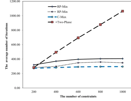
In table I, the boldface numbers identify that the smallest average number of iterations. The result in table I is plotted as in Fig.3.-6. RP-Min, RP-Max and C-Max identify three criteria: the smallest m1, the largest m1 and the largest coefficient of the objective function, respectively.

0.00 50.00 100.00 150.00 200.00 250.00 300.00 350.00 400.00 450.00

100 200 300 400 500

The

averag

e

num

b

er

of

i

te

ratio

ns

The number of constraints

[image:6.595.63.279.54.231.2]

RP-Min RP-Min C-Max Two-Phase

Fig. 4. The average number of iterations for ten variables.

0.00 200.00 400.00 600.00 800.00 1000.00 1200.00

200 400 600 800 1000

The

avera

ge

n

um

b

er

o

f

iteratio

ns

The number of constraints RP-Min

RP-Min C-Max Two-Phase

Fig. 5. The average number of iterations for 20 variables.

of iterations of the selected variable which has the largest coefficient of the objective function outperform two-phase method and another criteria.

V. CONCLUSIONS

In this paper, we proposed the artificial-free technique to improve the simplex algorithm. The objective plane can split constraints into three groups by considering the sign of coefficient for each constraint. Then constraints from the nonpositive groups (negative and zero coefficient groups) are relaxed. The relaxed problem can identify a feasible point by our theorem. Then it will be transformed for starting the sim-plex algorithm without using artificial variables. Constraints from the nonpositive groups are added for checking the solution from the relaxed problem. Since artificial variables is not used, the number of variables by our algorithm is less than or equal to the number of variables by the simplex algorithm. The number of constraints which solved by our algorithm is less-than or equal to the number of constraints which solved by the simplex algorithm. If all constraints contain in the group M1, then the number of constraints which solved by our algorithm and the simplex algorithm is equal. At each iteration, our algorithm solves partial tableau from the simplex tableau. So the dimension of parameters which used by our algorithm is less than or equal to the

0.00 200.00 400.00 600.00 800.00 1000.00 1200.00 1400.00 1600.00 1800.00 2000.00

300 600 900 1200 1500

The

average

n

um

ber

o

f

iteratio

ns

The number of constraints

RP-Min

RP-Min

C-Max

[image:6.595.317.539.62.235.2]

Two-Phase

Fig. 6. The average number of iterations for 30 variables.

dimension of parameters which the simplex algorithm used. This is one of the advantage of our algorithm. If the group

M1andM3is empty, then we can conclude that the original problem is unbounded without using the simplex algorithm. This is an obvious advantage of our algorithm. Moreover, we suggest the criteria to select the variable for mapping. From the computational results, we found that iterations from the selected variable which has the maximum cost of the objective function outperform the simplex algorithm, and another criteria.

REFERENCES

[1] M. S. Bazaraa, J. J. Jarvis and H. D. Sherali,Linear programming and network flows, 2nd edn. New York : John Wiley, 1990.

[2] H.V. Junior and M.P.E. Lins, “An improved initial basis for the Simplex algorithm,” Computers and Operations Research, vol. 32, pp. 1983– 1993, 2005.

[3] V. Klee and G. J. Minty, “How good is the simplex algorithm?,”

inequalities III, New York: Academic Press, pp. 159–175, 1972. [4] N. Karmarkar, “A new polynomial-time algorithm for linear

program-ming,” Combinatorica, vol. 4, 373–395, 1984.

[5] Wei-Chang Yeh, H.W. Corley, “A simple direct cosine simplex algo-rithm,”Applied Mathematics and Computation, vol. 214, pp. 178–186, 2009.

[6] H. Arsham, “An artificial-free simplex-type algorithm for general LP models,”Mathematical and Computer Modeling, vol. 25, pp. 107–123, 1997.

[7] H. Arsham, “Initialization of the simplex algorithm: an artificial-free approach,”SIAM Reviewvol. 39, pp. 736–744, 1997.

[8] A. Enge and P. Huhn, “A counterexample to H. Arsham’s “Initialization of the simplex algorithm: an artificial-free approach,SIAM Reviewvol. 40, online, 1998.

[9] P.Q. Pan, “Primal perturbation simplex algorithms for linear program-ming,”Journal of Computational Mathematics, vol. 18, pp. 587–596, 2000.

[10] H. Arsham, “Big-M free solution algorithm for general linear pro-grams,”International Journal of Pure and Applied Mathematics, vol. 32, pp. 37–52, 2006.

[11] H. Arsham, “A computationally stable solution algorithm for linear programs,”Applied mathematics and Computation, vol. 188, pp. 1549– 1561, 2007.

[12] H.W. Corley, Jar Rosenberger, Wei-Chang Yeh and T.K. Sung, “The cosine simplex algorithm,” The international journal of Advanced Manufacturing Technology, vol. 27, pp. 1047–1050, 2006.

[13] A. Boonperm and K. Sinapiromsaran, “The artificial-free technique along the objective direction for the simplex algorithm,” Journal of Physics: Conference Series, 490, pp. 1-4, 2014.

[image:6.595.58.282.270.443.2]