An Opportunistic Maintenance Decision of A
Multi-Component System Considering the Effect of
Failures on Quality
Pravin P. Tambe and Makarand S. Kulkarni
Abstract- Preventive maintenance is a planned activity to keep the manufacturing facilities in good condition. However, because of limited time and resources, not all the system components can be repaired/replaced during the planned opportunity. When the system is under maintenance, it is very conservative to take the maintenance decision on the components because of limited available time and resources, hence the decision is selective. In this paper, an approach for opportunistic maintenance of a multi-component system is presented. The objective is to obtain a minimum cost solution with required availability and which can be accomplished within the allowable maintenance time. The optimization of the proposed model in this paper results into maintenance decision in terms of maintenance actions namely, repair, replace or do-nothing for the system components. A genetic algorithm approach is used for getting the optimal solution. The application of the model is demonstrated through a case study of a high pressure die casting machine.
Keywords-Opportunistic maintenance, Multi-component system, Genetic algorithm, Rejection cost
Nomenclature
AReq : Required system availability
Β : Weibull shape parameter for component
η : Weibull scale parameter for component CC : Cost of component (Rs.)
Cf : Failure cost per incident for component (Rs.)
CLP : Cost of lost production (Rs.)
CLM : Labour cost of maintenance (Rs./hr)
Csp : Cost of sub-components and consumables (Rs.)
CR : Replacement cost for component (Rs.)
Cr : Repair cost for component (Rs.)
CRL : Cost of loss of residual life (Rs.)
E[DT]TPMS: Expected downtime in next operating period (hr.)
ML : Mean life (hr.) MRL : Mean residual life (hr.)
MTTrA : Mean time to repair for component (hr.) MTTRA : Mean time to replacement for component (hr.) MTTCA : Mean time to corrective action for component (hr.) PR : Production rate (units/hr.)
RF : Restoration factor for component
TPMS : Time between the current maintenance and
next expected opportunity (hr.)
TAvl : Time available to carry out maintenance (hr.)
Manuscript received March 18, 2013; revised April 05, 2013.
Pravin P. Tambe is a Research scholar in Mechanical Engineering Department at Indian Institute of Technology Delhi, Hauz Khas, New Delhi, India (email:[email protected], Ph No: +91-11-26596317, Mobile: +91-9811873959, Fax: 91-11-26582053)
Dr.Makarand S. Kulkarni is an Associate Professor in Mechanical Engineering Department at Indian Institute of Technology Delhi, Hauz Khas, New Delhi, India (email: [email protected])
TLM : Time elapsed between the last maintenance
and opportunity (hr.) TCf : Total cost of failures (Rs.)
TCR : Total cost of replacement (Rs.)
TCr : Total cost of repair (Rs.)
(vi)O : Effective age at opportunity (hr.)
I. INTRODUCTION
selective maintenance model to take maintenance decision considering limitation on maintenance time, budget and reliability of the system. Shalaby et al. [8] developed an optimization model for preventive maintenance scheduling of multi-component and multi-state system. They define the sequence of preventive maintenance activities as the decision variables and the summation of preventive maintenance, minimal repair, and downtime costs as the objective functions. Hu et al. [9] proposed an opportunistic predictive maintenance-decision method integrating machinery prognostic and opportunistic maintenance model to indicate the optimal maintenance time with minimal cost and safety constrains.
From the literature it is observed that, most of the models focus on identifying the criteria for maintenance opportunity and its cost effectiveness. Although, the machine condition affects the product quality, the effect of component failure and its consequence in terms of rejections is not generally considered in maintenance decision and the maintenance decision includes only maintenance related costs.
The objective of this paper is to develop an approach for opportunistic maintenance of a multi-component system to take an optimal maintenance decision by selecting maintenance actions for each component during a planned or an unplanned opportunity. A scheduled maintenance is considered as a planned opportunity, while any machine breakdown or stoppage due to other reason is an unplanned opportunity. The maintenance decision is based on the optimization of the total cost which includes all the direct and indirect costs like maintenance activity costs, residual life costs and future failure costs. The maintenance decision is taken considering the constraint on the available time for the maintenance actions, the system availability requirement in the next interval of system operation. The model also considers the effect of components failure on the quality of the product being manufactured and the cost of rejections is included in the total failure cost along with the maintenance and downtime cost.
In the next section, the system considered in this paper is presented.
II. SYSTEM DESCRIPTION
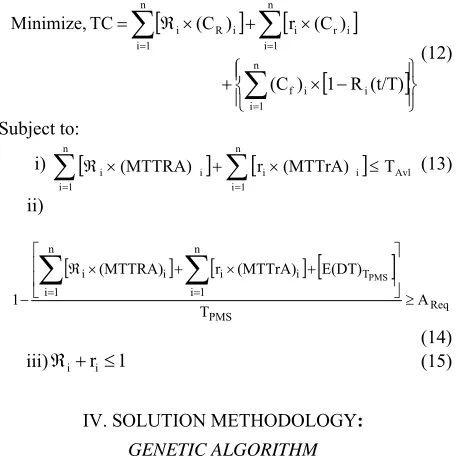
Consider a multi-component system having ‘n’ components, where each component is subjected to degradation due to continuous operation over a period of time and has an increasing failure rate (IFR). The time to failure distribution of each component is assumed to follow a two parameter Weibull distribution. The problem considered in this paper is shown in Fig. 1.
Fig.1. System description
The machine is available for maintenance after a time TLM
from the last maintenance action with each component in the system is having a certain age which depends on the last failure time. The next expected planned opportunity duration TPMS, which is the operating period for the
machine, is known. The maintenance decision needs to be optimized considering the system availability and the available time for maintenance. Since, all the system components cannot be subjected to maintenance due to limited resources and time, the decision is selective. For every component, one of the three actions namely, repair, replace and do-nothing is to be chosen. Even though the maintenance actions will improve the condition of the system, random failures may occur in the next period of operation. In this paper, we have considered two failure consequences associated with the component failures. The two failure consequences are:
1) Failure will lead to conditions where the detection is immediate and the machine needs to be stopped. This failure consequence is termed as FC1.
2) The failure is in terms of a degraded state where the machine will run, but lead to deterioration of the product quality being manufactured on the machine. This failure consequence is termed as FC2.
The failure consequence FC1 is immediately detectable while, the detection of FC2 is not immediate and occurs after a time lag. The magnitude of the time lag depends on the sensitivity of the quality control scheme. The objective is to obtain the maintenance decision with minimum total cost with required availability in the next period of system operation.
In the next section, model for the expected total cost for opportunistic maintenance is presented.
III. MODEL DEVELOPMENT
In this section, we develop an expected total cost model for opportunistic maintenance. Various aspects associated with the model and different cost components of the total cost are discussed in the following subsections.
A. Maintenance actions at an opportunity
For each opportunity, the model considers one of the following three types of maintenance actions:
i) Replacement action
In this category, during an opportunity, a component is replaced with a new one and the component starts its working with an age zero i.e. the restoration factor is ‘1’. ii) Repair action
In this category, during an opportunity, repair is carried out for a component. The maintenance action improves the condition of the component with an improvement factor and effectively its age is reduced. The restoration factor is between 0 and 1 for repair action. In the case of subsystems with a large number of components, repair usually results in replacing only a few of these. For such situations, it may be reasonable to assume minimal repair at the subsystem level i.e. RF=0.
iii) Do-nothing
In this category, no maintenance action is taken and the components are left as they are. For a given component, this could be because of the maintenance time constraint or it
1
2
n
TPMS
TLM
Current maintenance opportunity Last
maintenance
Next expected opportunity
System Component
Random failure
may be more cost effective to postpone the maintenance action to a future opportunity.
B. Residual life
Residual life is the remaining lifetime of a component which has survived up to certain duration of time (t’). The Mean Residual Life (MRL) of a component ‘i’, having survived a duration t’, can be expressed as (Ebeling, [10]),
∫
∞ = ) (t' i ii R(') R (t)dt
1 ) ' ( MRL t
t (1)
C. Cost of loss of residual life
When a component is preventively replaced at an opportunity, the effect of the loss of residual life is considered. The cost due to the loss of residual life (CRL) will be proportional to the cost of the component. If we assume that the component cost is uniformly distributed over the lifetime of the component, the cost due to the loss of residual life will be given by,
i i i i MRL ML CC
CRL = × (2)
where, MLi is the mean life ,
∫
∞=
0 i i R(t)dt
ML
D. Cost of replacement
If a component is replaced at an opportunity, the cost of replacement incurred will be given by,
] CRL CC ) C C (PR [MTTRA )
(CR i= i× × LP+ LM + i+ i (3)
where , MTTRA is the mean time to replacement action. Therefore, the expected total cost of replacement (TCR) at an
opportunity considering all the candidate components is given by,
( )
[
]
∑
= × ℜ = n 1 i i R i R CTC (4)
⎩ ⎨ ⎧ = ℜ otherwise. 0, replaced. is component i if 1, where, th i
E. Cost of repair
If a component is repaired at an opportunity, the cost of repair for the ith component will be given by,
( )
C ] ) C C (PR MTTrA [ )(Cr i= i× × LP+ LM + sp i (5)
where, (Csp)i is the cost of consumables during the repair of
ith component.
Therefore, the expected total cost of repair (TCr) at an
opportunity considering all the candidate components is given by,
[
]
∑
= × = n i1 i r ir r (C )
TC (6)
⎩ ⎨ ⎧ = otherwise , 0 repaired is component i if , 1 r where, th i
F. Total cost of failure
The failure of a component can result into two possible Failure Consequences (FC). It can either immediately bring the machine under breakdown indicating total failure or the machine will operate, but affect the quality of the product being manufactured. The failure consequences are termed as FC1 and FC2 respectively. The detection of FC2 may not be immediate and occur after a time lag with the aid of process monitoring mechanisms like control charts or other sampling procedures. However, from the time of occurrence of the failure till its detection, the process operates in a degraded condition which leads to higher levels of rejection or rework.
In this paper, the cost of failure is considered as the cost associated with the repair/replace actions, downtime cost and the cost of rejection on account of quality. In other words, the cost of failure is a consequence of the maintenance actions chosen at an opportunity over the next period of operation i.e. till the next expected scheduled opportunity. In the present study, the expected downtime, E(DT) over a given period is determined through a failure simulation approach using the time to failure distribution of the component (Yanez et al. [11]) and the corresponding corrective action time.
( )
[
( )
]
∑
= − × = n 1 i i i ff C 1 R t/T
TC (7)
where, (Cf)i is the cost of failure of the ith component and is
given by, ] C r CC ) C C (PR [MTTCA )
(Cf i= i× × LP+ LM +ℜi× i+ i× spi
+(PR×IRR×TTDFC2×CRej)×QFi
(8) where, repaired. is component i if , MTTrA replaced. is component i if , MTTRA MTTCA th i th i i ⎪⎩ ⎪ ⎨ ⎧ = ⎩ ⎨ ⎧ = otherwise. 0, quality. product affect component i of failure if 1, QF th i
The expected time to detect the occurrence of failure consequence FC2 is calculated from the average run length parameter of the quality control scheme.
interval sampling β -1 1 TTD S
FC2= × (9)
where, βS = Type 2 error of quality control scheme.
G. Total maintenance cost
The total cost incurred due to an opportunistic maintenance decision is the sum of maintenance cost and total failure cost which is given as,
f
M TC
TC
[
]
[
]
[
]
⎪⎭ ⎪ ⎬ ⎫ ⎪⎩ ⎪ ⎨ ⎧ − × + × + × ℜ =∑
∑
∑
= = = n 1 i i i f n 1 i i r i n 1 i i R i (t/T) R 1 ) (C ) (C r ) (C TC (11)H. Optimization of model
For the maintenance optimization of a multi-component system, efficient maintenance decisions should be taken whenever opportunity arises. The objective of the optimization is to generate a set of maintenance decisions that will lead to a minimum total cost while meeting all the constraints. The objective function considered in the present study for the optimization of the maintenance decision is as follows:
[
]
[
]
[
]
⎪⎭ ⎪ ⎬ ⎫ ⎪⎩ ⎪ ⎨ ⎧ − × + × + × ℜ =∑
∑
∑
= = = n 1 i i i f n 1 i i r i n 1 i i R i (t/T) R 1 ) (C ) (C r ) (C TC Minimize, (12) Subject to:i)
[
]
n[
]
Avl1 i i i n 1 i i
i×(MTTRA) + r ×(MTTrA) ≤T
ℜ
∑
∑
= = (13) ii)[
]
[
]
[
]
Req PMS T n 1 i i i n 1 i i i A T E(DT) (MTTrA) r (MTTRA) 1 PMS ≥ ⎥ ⎥ ⎦ ⎤ ⎢ ⎢ ⎣ ⎡ + × + × ℜ −∑
=∑
= (14) iii)ℜi+ri≤1 (15)IV. SOLUTION METHODOLOGY:
GENETIC ALGORITHM
Genetic Algorithms (GAs) are adaptive search techniques based on the evolutionary ideas of natural selection and genetics (Goldberg [12]). GA has been used in a wide variety of applications, particularly for finding the global optimum solution for an optimization problem. A Genetic algorithm works on the principle of survival of the fittest by progressively accepting better solutions to the problems. It operates on the population of potential solutions to the problem and iterates towards the optimum solution. As the search iterates, the population includes fitter solutions converging towards the near-optimality. The basic elements of genetic algorithm are solution representation, population, evaluation (Fitness), selection, crossover and mutation. The crossover and mutation are considered to be the main operators of GA. The algorithm starts with a randomly generated initial set of population consisting of chromosomes, which represent the solution of the problem. The chromosomes are evaluated for the fitness function or the objective function and selected according to their fitness value. The selected chromosomes then undergo crossover and mutation operation with a certain probability to form new generations. The general mechanism of a genetic algorithm is shown in Fig. 2.
Fig. 2. General mechanism of GA
V. ABOUT CASE STUDY
A real life case study of High Pressure Die Casting (PDC) machine is considered for demonstrating the opportunistic maintenance methodology proposed in this paper. The company being considered is a first tier supplier of pressure die cast (PDC) components to automobile OEMs in India and abroad. The company has a large PDC section containing 35 machines of different capacities. The data of one of the machines has been used to demonstrate the proposed methodology. The machine under consideration operates for 7 hours per shift and 3 shifts per day. The details of the components which are considered for maintenance are given in Table I. (NA in Table I indicates ‘not applicable’)
The production rate is 72 units per hour and the profit is Rs. 8 per piece. The labor cost for maintenance is Rs. 100 per hour. The minimum required availability in the next operating period is 0.95. In the present case study, the same sampling plan, which is used by the company for quality control purpose is considered, where the sample size is 1, the time between samples is 1 hour and the acceptance number is 0. From the shop floor records it was observed that, failure of five machine components (Sr. no 22-26 in Table I) leads to increase in the defective rate. The normal defective percentage is 8% while in the case of failure of these five components, the defective rate increases to 20 %. If the sample size is 1 with an acceptance number of 0, the probability of not detecting a failed state at any given sample is 0.8, which is the type 2 error and hence, it will take 5 samples on an average to get an indication of a process failure. Since the time between samples is 1 hour, the time to detect the occurrence of failure consequence (FC2) will be 5 hours in the present case. From this, the increase in the rejection cost is calculated. The details of the components whose failure affect the product quality and results into an increase in the defective rate are given in Table I (Sr. no. 22-26). In the present case, whenever any of these components fail, it results into blow holes and non-filling in the castings. However, it should be noted that the given increase in the defective rate is specific to the machine under consideration.
Begin GA
Create Initial population (Chromosomes) Select Fitness function.
Evaluate each chromosome. while (termination criteria)
Selection- of the stronger chromosomes as parents. Crossover -mate the chromosomes to form offsprings with a probability of crossover.
Mutation- mutate the offsprings with a probability of mutation.
Evaluate the fitness of new population. end
[image:4.612.313.529.54.203.2] [image:4.612.73.301.223.451.2]TABLE I
MAINTENANCE DATA FOR MACHINE COMPONENTS
Sr.
No Component β η (hr.)
Component cost during replacement
(Rs.)
Failure cost (Rs.)
Sub-component/ consumables
cost during repair (Rs.)
MTTrA (hr.) MTTRA (hr.)
1 Electrodes 1.61 2388 1100 776 100 1 0.33
2 Electrode
Insulator 1.07 3458 100 776 NA NA 1
3 Electric wire 1.06 7877 300 976 NA NA 1
4 Arm Bearings 2.83 1837 6200 6538 200 1 0.5
5 limit switch 3.33 14027 20000 20676 NA NA 1
6 Chain 6.04 1623 5000 2352 800 2 3
7 Chain lock 4.14 3368 150 826 NA NA 1
8 Bearing (cup
side) 2.83 1837 2500 5028 200 1 3
9 Pneumatic Cylinder 3.33 14027 30000 31402 NA NA 2
10 Seal 4.40 6680 7000 8352 NA NA 2
11 Dia. Valve 5.56 3265 8000 9352 NA NA 2
12 connector 2.49 7738 250 473.08 NA NA 0.33
13 Shock Absorber 3.33 14027 10000 10676 NA NA 1
14 Valve screw 2.59 22803 100000 12028 10000 3 4
15 Gear box 3.93 20364 100000 18760 12000 10 4
16 Servo valve 3.33 14027 200000 200676 200 4 1
17 Inj. Unit piston 3.93 20364 160000 192448 20000 8 48
18 Shot sensor 3.76 6840 100000 105338 NA NA 0.5
19 Teflon seal 5.94 1624 150 319 NA NA 0.25
20 Extractor
Bearings 2.69 14027 12200 17608 NA NA 8
21 length adjustor 4.64 9958 250 926 50 1 1
22 Acc. Piston 2.69 3744 120000 60292 50000 5 6
23 Acc. seal 2.83 1837 50000 59616 NA NA 4
24 safety valve 3.01 36023 10000 8088 500 1 1
25 O'ring Set 3.33 14027 40000 55700 NA NA 13
26 Couplings 2.49 7738 16200 11492 1000 5 1
VI. RESULTS OF OPTIMIZATION
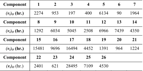
In order to demonstrate the applicability of the proposed model, a scheduled maintenance is considered as a maintenance opportunity. The time between last maintenance and current opportunity is taken to be 800 hours and the time till next scheduled opportunity is 1000 hours. It is assumed that 20 hours are available for the maintenance work. The maintenance decision should be taken for the system such that the maintenance actions should be completed within this time and meet the target availability requirements. The effective age values of the components at the opportunity are given in Table II. The age values indicates the deterioration of the system components from the last maintenance and continuous operation till the current opportunity. The opportunistic maintenance approach proposed in this paper is applied and the possible maintenance actions for the system components will be evaluated at this maintenance opportunity, using genetic algorithm (GA) as the solution methodology.
TABLE II
EFFECTIVE AGE OF COMPONENTS AT THE OPPORTUNITY
Component 1 2 3 4 5 6 7
(vi)O (hr.) 2274 953 197 400 6134 90 1964
Component 8 9 10 11 12 13 14
(vi)O (hr.) 1292 6034 5045 2508 6966 7439 4350
Component 15 16 17 18 19 20 21
(vi)O (hr.) 15481 9696 16494 4452 1391 964 1224
Component 22 23 24 25 26
(vi)O (hr.) 2401 621 28495 7109 4530
[image:5.612.311.545.506.623.2]chromosomes, which is generated randomly, a crossover probability of 0.8, a mutation probability of 0.05 and the total number of generation as 2000. The total cost of the maintenance decision is used as a fitness function for evaluating the relative fitness of each maintenance decision. A roulette wheel selection method is used for the chromosome selection and a two point crossover is used to form new off-springs during the crossover operation. The results of the maintenance decision using the GA are given in Table III and the path taken by the total cost during the generations is shown in Fig. 3.
TABLE III
RESULTS OF MAINTENANCE DECISION USING GA.
Maintenance Action
Repair Components - Nil Replace Components- 7,8,19
Do Nothing
Components- 1,2, 3, 4, 5, 6, 9, 10, 11, 12, 13, 14, 15, 16, 17, 18, 20, 21, 22, 23, 24, 25,26
Total Cost
(Rs.) 215535
Maintenance decision Cost(Rs.)
4360
Future Risk
(Rs.) 211175
Availability 0.9562
Time taken 592.317 seconds.
Fig. 3. Total cost progress over generations.
VII. CONCLUSION
This paper has presented an approach for opportunistic maintenance of a multi-component system. A cost model considering the expected total cost of maintenance decision with the constraints of availability and allowable maintenance time is developed. A genetic algorithm approach is used for optimization of the maintenance decision. Optimization of the proposed model results into maintenance decision by taking one of the three maintenance actions namely, repair, replace or do-nothing for the system components. The approach presented in this paper, is practical to implement on the shop floor and will help maintenance managers to effectively evaluate the maintenance actions based on the condition of the system components. It will also aid to effectively manage the resources such as manpower, spares etc. As a future research scope, the other solution methodologies can be applied to
obtain the optimal solution and their performance can be compared.
REFERENCES
[1] L. Cui and H. Li, “Opportunistic maintenance for multi-component shock models.” Mathematical Methods of Operations Research, vol. 63, no. 3, pp. 493–511, 2006
[2] X. Zheng and N. Fard, “A maintenance policy for repairable systems based on opportunistic failure-rate tolerance.” IEEE Trans. on Reliability , vol.40, no. 2, pp.237-244, 1991
[3] A.S.B. Tam, W. Chan M and J.W.H. Price Maintenance scheduling to support the operation of manufacturing and production assets, International Journal of Advanced Manufacturing Technology, vol. 34, pp. 399–405, 2007
[4] M.S. Samhouri, “An intelligent opportunistic maintenance (OM) system: A genetic algorithm approach” IEEE Int. Conf. Science and Technology for Humanity (TIC-STH), pp.60-65, 2009
[5] X. Zhou, L. Xi and J. Lee, “Opportunistic preventive maintenance scheduling for a multi-unit series system based on dynamic programming” International Journal of Production Economics , vol. 118, no. 2, pp. 361-366, 2009
[6] H. Saranga, “Opportunistic maintenance using genetic algorithms", Journal of Quality in Maintenance Engineering, vol. 10, no. 1, pp. 66-74. 2004
[7] C.R. Cassady, E.A. Pohl and W. Paul Murdock Jr., “Selective maintenance modelling for industrial systems” Journal of Quality in Maintenance Engineering, vol. 7, no.2 pp. 104-117, 2001.
[8] M.A. Shalaby, A.H. Gomaa and A.M. Mohib, “A genetic algorithm for preventive maintenance scheduling in a multiunit multistate system” Journal of Engineering and Applied Science, vol.51 no. 4, pp. 795–811. 2004.
[9] J. Hu, L. Zhang and W.Liang, “Opportunistic predictive maintenance for complex multi-component systems based on DBN-HAZOP model “ Process Safety and Environmental Protection, v ol. 90, no. 5, pp. 376–388, 2012
[10] C.E. Ebeling An introduction to reliability and maintainability engineering. Tata McGraw -Hill Education Private Limited, New Delhi (India), 2010
[11] M. Yanez, F. Joglar and M. Modarres, “Generalized renewal process for analysis of repairable systems with limited failure experience” Reliability Engineering & System Safety , vol.77, no. 2 , pp. 167-180, 2002
[12] D. Goldberg Genetic algorithms in search optimization and machine learning. Addison-Wesley, New York, 1989
T
otal C
ost (R
s.)