Abstract—Most of the inventory models under supply disruptions are based on the assumption that either the failure process is time-independent or the system is perfectly repaired after each failure. However, in the real situation, the failure process can be time-dependent and the supplier can also perform imperfect repairs. In this work, we study deterministic demand (Q, r) inventory models under time-dependent disruption due to machine breakdowns at the supplier with the possibility that a repair after each failure is imperfect.
Index Terms—Inventory model, imperfect repair
I. INTRODUCTION
Inventory problem under supply disruptions is widely studied in recent years. The reasons why this problem is important is because in reality the suppliers can be unavailable from time to time due to several disruptions such as natural disasters, machine breakdowns, labor strikes, terrorisms, etc. In these situations, the firm, the customer, need effective strategies to cope this problem in order that the business can run smoothly. Most of the inventory models under supply disruptions are based on the assumption that the failure rate and the repair rate are constant and independent of time. Under this assumption, the time to 1st failure and the repair time are exponentially
distributed random variables. This assumption is convenient for the model formulation and the computation, for the Markov property is conserved. By contrast, time dependent problems are often non-Markovian, which are more complicated than the Markovian counterparts. However, the assumption of time-independence is not practical for many situations. One of such situations is that when the disruptions occur due to machine breakdowns. There are three main reasons that make the exponential model impractical in generalization disruptions due to machine breakdowns. First, normally, machines deteriorate with time. Older machines incline to fail more often than newer machines. Second, the repair time are practically not exponentially distributed. Third, the exponential model is based on the assumption that the repair is perfect, that is, each repair brings a machine back to the brand-new condition. Generally, this assumption is seldom true, for the
This manuscript is submitted on 7th Jan 2014
Thanawath Niyamosoth is with Academy of Mathematics and System Sciences Chinese Academy of Sciences, Beijing, PR China (e-mail: [email protected])
Ya-Xiang Yuan is with Academy of Mathematics and System Sciences Chinese Academy of Sciences, Beijing, PR China (e-mail: [email protected])
general repair of machine is often imperfect. Namely, after each repair, a machine becomes younger, in terms of failure rate, but not brand-new. In our work, by applying the theory of non-homogeneous Markov chain, we propose a model for the inventory problem under time-dependent disruptions due to machine breakdowns that the Markov property is conserved. Moreover, we also consider the effect of imperfect repairs, which is overlooked by other publications, in our model as well. The results show that the assumptions about the failure rate functions, the repair rate functions, and the degree of imperfect repairs have significant impact on the optimal solutions of the model.
II. MODELFORMULATION In our work, we use the following notation:
Q
= order quantityr
= reorder pointt
= time to 1st occurrence of failure or repair
t
= failure rate function
t
= repair rate functionc
= corrective maintenance coefficientD
= demand rateK
= fixed ordering cost per orderh
= holding cost per unit per time
= backorder cost per unit backordered
ˆ
= backorder cost per unit per timey
= repair time
y
g
= probability density function ofy
A. Failure and Repair Rate Function
In our work, we define failures as non-homogeneous Poisson process (NHPP), which is a Markov process, with Weibull failure rate as the following.
;
0
,
0
,
0
1
t
t
t
(1)
is called the shape parameter, and
is called the scale parameter respectively. Note that when
1
, the failure rate is constant as in the exponential case. When
>1, the model becomes an increasing failure rate case, generalizes the deterioration process of the machine. The repair rate function is defined as:
;
0
,
0
,
0
1
t
t
t
(2)
(Q, r) Inventory Model under Supply
Disruptions and General Repairs
Similar to the failure rate function,
is the shape parameter, and
is the scale parameter respectively. When1
0
, the repair rate is an decreasing function, when1
, the repair rate is constant as in the exponential case, and when
1
, the repair rate function is decreasing. Note that even though the exponential repair is applied widely in many publications; however, in reality, the repair time is seldom exponentially distributed. In the next section, we develop the two-state non-homogeneous Markov chain of the problem.B. Two-State Non-Homogeneous Markov Chain of ON/OFF Period
The system is in ON period when the machine is operating and OFF when the machine is down. If a perfect repair at each failure is assumed, when the system is ON, it will move to OFF period with rate
t
, and when the system is OFF, it will move to ON with rate
t
. If at each failure a repair is perfect (as good as new) with probabilityp
, and with probability1
p
a repair is minimal (as bad as old), then the resulting failure rate due imperfect repairs is:
;
0
c
1
,t
0
c
t
λ
t
λ
I (3)Proof.
Assume that a machine has been used for
t
1, then it fails. If a repair is perfect, then the failure rate function after a perfect repair will be
t
. If a repair is minimal, then the failure rate after a minimal repair will be
t
t
t
. Thus, the failure rate after an imperfect repair is defined as
t
p
t
1
p
t
t
1
I
. So,
I
t
is on theline joining
t
and
t
t
1
. We can rewrite
I
t
as
t
λ
t
α
λ
t
t
1
λ
t
;
0
α
1
λ
I . Divide
t
I
by
t
, we get
t
t
t
t
t
t
I
1
1
.Because
t
t
1
t
0
, thenλ
I
t
a
λ
t
; a
1
. Leta
c
1
, then we have
;
0
c
1
c
t
λ
t
λ
I .Proved. Note that if we relax the condition
0
c
1
by allowingc
1
, then the repair will be perfect. In our work, we define the failure and the repair process as a two-state non-homogeneous Markov chain as in Fig. 1Fig. 1 Two-state non-homogeneous Markov chain for imperfect repair
Let
p
01
v
,
t
be the transition probability that the system is in state 0 (ON) at timev
and will move to state 1 (OFF) at timet
. By applying Kolmogorov’s forward equation,
v
t
p
01,
can be found by solving the following differential equation.
,
0
1
0
01
01
,t
c
;
c
t
λ
t
μ
c
t
λ
v,t
p
t
t
v
p
(4) Becauset
= time to 1st failure, then we letv
0
. Thus, bystandard calculus methods, we have
0
1
0
0
0 0
0
01
,t
c
;
e
dx
e
c
x
λ
,t
p
t x dx x μ c x λt μx dx
c x
λ
(5) Thus, we can find the probability that the system is in state 0 at time 0 and in state 1 at time
t
by calculatingp
01
0
,
t
. Note that when
1
, the failure rate is constant, that is
t
. In this case the failure distribution reduces itself into the exponential case with
1
. Likewise, when1
, the repair rate is constant, that is
t
1
.Therefore, the transition probability,
p
01
0
,
t
, reduces itself into
1
0
0
0
01
;
λ
,
μ
,t
e
μ
λ
λ
t
p
λ μt as inthe case of the standard two-state homogeneous Markov chain. However, we can see that, in the non-homogeneous case, the calculation of
p
01
0
,
t
by solving Kolmogorov’s forward equation is burdensome. This obstacle can be overcome by using the approximation method as described in [1]. In this method, we define the reliability function
t
Pr
T
t
; t
0
R
which represents the probabilitythat a machine will not fail before time
t
. Letf
t
be a probability density function oft
, the we can define the failure rate function
t
, forc
1
, as the following:
t
R
t
f
t
t
T
t
t
T
t
t
t
lim
0Pr
/
Let
F
t
be a cumulative distribution function oft
, the
t
F
t
R
1
. Thus,
t
R
t
R
t
R
t
F
t
' '
, then we
tx
dx
t
R
0
exp
. Let
t
dx
x
t
0
be thecumulative failure intensity function, then we have
t
exp
Λ
t
; t
0
R
. By definition,R
t
is the probability that starting from time 0 a machine will not fail at leastt
. Thus,R
t
is the probability that starting from ON state at time 0, the system is still ON at time t. Let
t
p
000
,
be the probability that at time 0 the system is ON and is still ON at timet
. Then,
t
R
t
t
p
000
,
exp
. From Markov chain, we know thatp
00
0
,
t
p
01
0
,
t
1
. Thus, we can find the transition probabilityp
01
0
,
t
from the followingequation:
0
1
exp
0
01
,t
Λ
t
; t
p
(6)Where
t
c
dx;
c
x
λ
t
Λ
01
0
for imperfect repair. C. The Objective FunctionIn this section, we continue to the formulating of the inventory model. The objective of this work is to find the order quantity
Q
and the reorder pointr
that minimize the objective function in, the average annual cost, which can be found by applying the renewal reward theorem as in the following equation.
Cycle
length
E
cycle
per
costs
Total
E
Cost
Annual
Average
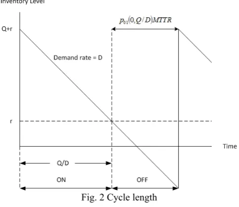
(7)D. Cycle Length
Assuming that lead time is zero, the cycle starts when the system is ON and the inventory level is
Q
r
. When the inventory level hits the reorder point,r
, at timeQ
/
D
, with probabilityp
01
0
,
Q
/
D
the system will be OFF for the average duration ofMTTR
whereMTTR
= mean time to repair which can be found from
1
1
MTTR
where
x
is Gamma function ofx
, and
is the scale parameter of Weibull repair time. Therefore, we can calculate the expected cycle length,
CL
E
, by the following equation.
p
Q
D
MTTR
D
Q
/
,
0
CL
E
01 (8)This means the cycle lasts at least
Q
/
D
and with [image:3.595.100.539.42.791.2] [image:3.595.306.548.55.264.2]probability
p
01
0
,
Q
/
D
it will last for anotherMTTR
. Fig. 2 illustrates the cycle length of the model.Fig. 2 Cycle length D. Total Costs Per Cycle
The total costs in a cycle can be divided into two period (i) costs occurring in ON period (ii) costs occurring in OFF period.
(i) Expected Costs in ON Period
There are two costs in ON period, first fixed ordering cost and second holding cost. The expected costs in ON period can be calculated from the following equation.
D
hQr
D
hQ
K
N period
Costs in O
E
2
2
(9) (ii) Expected Costs in OFF period
There are two costs in OFF period, first holding cost and second backorder cost. The amount of costs in this period depends on two factors. The first factor is the reorder point. The second factor is the time used for repairing the machine. Let
r
be the reorder point, andy
be the Weibull repair time with pdf.
1
0
0
0
,y
,
;
ψ
e
y
ψ
y
g
y/ ψψ
(10)Let
C
10
r
,
y
be the random variable representing the costs occurring in OFF period which is the function ofr
andy
and can be defined as:
0 2 ˆ 2 0 0 2 2 2 2 10 ,r D r ; y D r yD π r yD π D hr ,r D r y ; D y ry h r,y C (11) Hence, we can calculate the expected costs in OFF period from the following equation.This cost occurs with the probability
p
01
0
,
Q
/
D
, then by combining all costs, we obtain the expected total costs per cycle,E
TC
, as follows.
p
Q
D
E
C
r
y
D
hQr
D
hQ
K
T
E
0
,
/
,
2
C
01 102
(13) E. Optimization Problem
By applying the renewal reward theorem, we obtain the objective function, the average annual costs,
AC
Q
,
r
, as follows.
; Q
0
,r
0
CL
E
TC
E
Q,r
AC
(14)Hence, the optimization problem in our research is:
0
0
,r
Q
Q,r
Min AC
(15)
III. NUMERICALEXAMPLE
In this section, we provide the results of the problem and the sensitivity analyses. The software that we use is Mathematica 9. The test parameters are borrowed from [11] except we use D = 10 in our test. Other parameters are K = $10/order, h = $5/unit/year,
= $250/unit,
ˆ
= $25/unit/year, EOQ =2KD/h
= 6.32456 units, REOQ =0. The test results are shown in the following tables. Table. 1 (a) Test results 1
θ = 4, c = 1
ψ = 1, φ = 0.4
β = 1 β = 1.5 β = 2 AC(Q*,r*) 95.3531 80.2664 59.303
r* 9.61317 5.8488 0.546079
Q* 6.57972 4.8404 3.54486
AC(EOQ, 0) 249.072 126.933 71.1124 AC(QEXP, rEXP) 95.3531 86.7072 86.6718
Table. 1 (b) Test results 1 (cont.)
θ = 4, c = 1
φ = 0.4
β = 2.5 β = 3 β = 4 AC(Q*,r*) 42.993 36.4991 32.5219
r* 0 0 0
Q* 4.2252 4.94934 5.85912
AC(EOQ, 0) 47.5907 38.0151 32.6373 AC(QEXP, rEXP) 80.9344 80.2122 79.7958
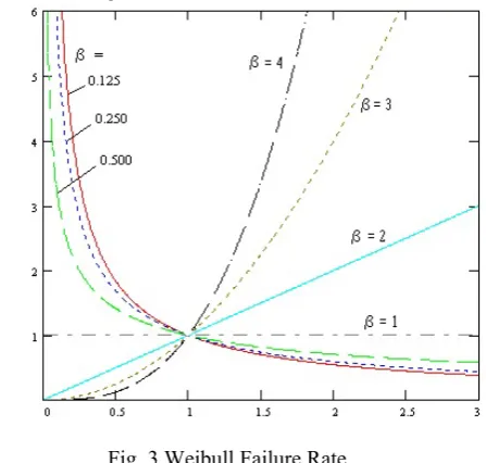
The results show that the shape parameter β has a significant impact on the optimal solution. Most publications in the literature assume that the failure rate is constant, that is β = 1 in our model; however, we can see that this assumption leads to great error. For example, it the failure rate is not constant but increasing with β = 2, the assumption of constant failure rate incurs 46% cost error. Another observation is that when β increases, the reliability of the system improves. We can see that the optimal safety stock r* and the optimal annual costs reduce significantly. Also, when β is large the problem approaches EOQ case. The reason for this result is that for larger β, the failure rate
function increases from zero slower than that of the smaller
[image:4.595.322.546.74.287.2]β as shown in Fig. 3.
Fig. 3 Weibull Failure Rate
[image:4.595.296.550.317.420.2](http://www.mathpages.com/home/kmath122/kmath122.htm)
Table. 2 Test results 2 β =1.5
c = 1 ψ = 1 φ
= 0.4
θ = 2 θ = 3 θ = 4 θ = 5 θ = 6
AC (Q*,r*)
96.3861 87.46 80.2664 74.3496 69.3547
r* 9.74226 7.5 5.8488 4.5817 3.47682 Q* 5.20167 4.94994 4.8404 4.78193 4.74654
Table. 2 shows the effect of θ on the optimal solutions. We can see that as θ increases AC(Q*,r*) and r* decrease significantly while when θ decreases the effect is opposite. The reason for this phenomenon is that increasing of θ
[image:4.595.41.289.414.633.2]reduces mean time between failure (MTBF). Because the failure process in our work is based on time to first failure, so in this case MTBF = MTTF = Г(1+1/β)θ. Therefore, when θ increases, MTTF also increases leading to the increasing of the reliability of the system.
Table. 3 Test result 3
β = 1, θ = 4 c = 1, φ = 0.4
AC(Q*,r*) r* Q* r*/Q*
ψ = 0.5 171.598 5.53715 2.03447 2.7217
ψ = 0.6 127.708 6.16996 2.92583 2.1088
ψ = 0.7 106.442 6.26103 3.63021 1.7247
ψ = 0.8 94.0086 6.16223 4.15774 1.4821
ψ = 0.9 85.9175 6.00834 4.54824 1.3210
ψ = 1.0 80.2664 5.8488 4.8404 1.2083
[image:4.595.296.556.554.681.2]failure to consider time-dependent repair rate leads to suboptimal solution. For example, if we assume ψ = 1 when it is in fact 0.5, then AC(QEXP, rEXP) = 194.35 which is
[image:5.595.315.563.231.681.2]larger than the optimal solution of 171.598. Another observation is that when ψ increases, the r*/Q* ratio reduces. This implies that when ψ increases the firm tends to use running stocks instead of safety stocks to fulfill customer demands.
Table. 4 Test results 4
β = 1.5,
θ = 4,
ψ = 0.5 c = 1
AC(Q*,r*) r* Q* r*/Q*
φ = 0.1 68.3704 2.09849 4.43573 0.4731
φ = 0.2 103.709 3.5781 3.24959 1.1011
φ = 0.3 137.709 4.67139 2.51461 1.8577
φ = 0.4 171.598 5.53715 2.03447 2.7217
φ = 0.5 204.817 6.26318 1.70161 3.6807
φ = 0.6 237.843 6.8987 1.45894 4.7286
φ = 0.7 270.809 7.4731 1.27477 5.8623
φ = 0.8 303.806 8.00509 1.13046 7.0813
φ = 0.9 336.899 8.50723 1.01444 8.3861
φ = 1.0 370.133 8.98834 0.919199 9.7784 The results in Table. 4 show the effect of φ, the scale parameter of the repair time, on the optimal solutions. The conclusion we deduce from the test is that when φ increases, the optimal average annual costs, AC(Q*,r*), and the optimal safety stock, r*, also increase because mean time to repair (MTTR) increase. Also, the r*/Q* increases as φ
increase. This implies that if the mean time to repair is long, the firm tends to fulfill the demand by using safety stock.
Table. 5 Test results 5
β = 1.5
θ = 4
ψ = 0.5
φ = 0.4
AC(Q*,r*) r* Q*
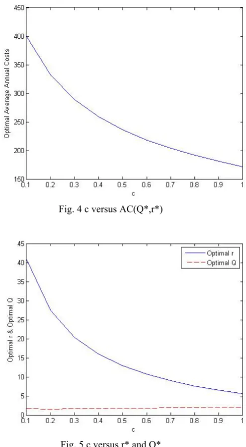
c = 1.0 171.598 5.53715 2.03447 c = 0.9 180.732 6.45996 1.97788 c = 0.8 191.273 7.57848 1.91961 c = 0.7 203.617 8.95754 1.85958 c = 0.6 218.347 10.6958 1.79776 c = 0.5 236.356 12.9524 1.7344 From the results in Table. 5, we can see that as c, the corrective maintenance coefficient, decreases, the average annual costs increase. By contrast, the average annual costs decrease when c increases. Note that the repair at each failure is perfect when c = 1. The conclusion for these results is that not only the failure and repair rate that have a significant impact on the optimal solutions but also the corrective maintenance action performed at each failure as well. If the supplier inclines to perform perfect maintenance more often than minimal repair, c will be closer to 1. On the other hand, if the supplier inclines to perform minimal repair more often and perform perfect repair less often, the coefficient c will more divert from 1. Failure to consider the
degree of corrective maintenance action at each failure leads to significant loss. For example, if the firm, the customer, assumes that a perfect repair is performed by the supplier at each failure when it is in fact that the supplier performs imperfect repair with c = 0.5 at each failure, AC(Q, r) will be 252.99 instead of 171.598 as the firm first expects. Another observation is that when c decreases, r* increases significantly. This implies that the firm tends to fulfill the demand by using safety stocks when repairs divert from perfect repairs. One the other hand, if repairs incline to be perfect, that is c increases, the firm tends to reduce the safety stock; thus, r* decreases. The effect of c on the optimal solution can be illustrated in Fig. 4 and Fig. 5.
Fig. 4 c versus AC(Q*,r*)
Fig. 5 c versus r* and Q*
IV. CONCLUSION
[image:5.595.43.298.475.615.2]imperfect corrective maintenance on the optimal solutions. Numerical tests show that the assumptions about failure and repair rates as well as the degree of imperfect corrective maintenance at each failure have significant impacts on the optimal solutions.
REFERENCES
[1] O. O. Aalen, O. Borgan, H. K. Gjessing, Survial and event history analysis: a process point of view, New York: Springer, 2008. [2] E. Berk, A. Arreola-Risa, “Note on future supply uncertainty in EOQ
models,” Naval research logistics, 41, 1994, 129-132.
[3] W. R. Blishchke, D. N. P. Murthy, Rliability, modeling, prediction and optimization, New York: John Wiley & Sons, 2000.
[4] M. Brown, F. Proschan, “Imperfect maintenance,” Survival Analysis: Proceeding of the special topics meeting sponsored by the institute of mathematical statistics, October 16-28, 1981, 179-188.
[5] M. Brown, F. Proschan, “Imperfect repair,” Journal of applied probability, 20, 1983, 851-859.
[6] R. L. Dobrushin, “Generalization of Kolmogorov’s equations for Markov processes with finite number of possible states,” Mat. Sb (N.S.), 33(75):3, 1953, 567-596.
[7] C. E. Ebeling, An introduction to reliability and maintainability engineering, Illinois, Waveland, 2010.
[8] J. Jaturonnatee, D. N. P. Murthy, R. Boondiskulchock, “Optimal preventive maintenance of leased equipment with corrective minimal repairs,” European journal of operational research, 174, 2006, 201-215.
[9] M. Parlar, “Continuous-review inventory problem with random supply interruptions,” European journal of operational research, 99, 1997, 366-385.
[10] M. Parlar, D. Berkin, “Future supply uncertainty in EOQ models,”
Naval research logistics, 38, 1991, 107-121.
[11] M. Parlar, D. Perry, “Inventory models of future supply uncertainty with single and multiple suppliers,” Naval research logistics, 43, 1996, 191-210.
[12] A. M. Ross, Y. Rong, L. V. Snyder, “Supply distributions with time-dependent parameters,” Computer and operations research, 35(11), 2008, 3504-3529.
[13] S. M. Ross, Stochastic processes, John Wiley & Sons, 1996. [14] K. S. Trivedi, Probability and statistics with reliability queuing and
computer sciences applications, John Wiley and Sons, 2002. [15] N. Yang, B.S. Dhillon, “Availability analysis of a repairable standby