Abstract—TCP/IP networks should have a good
management of congestion: users require fast and reliable communications. Congestion is more difficult to detect if there are wireless links, as the network delays and the number of users change constantly, so transmission problems arise. Typically, congestion is handled with drop tail or random early detection (RED) algorithms, although automatic control techniques are already giving good solutions. This paper presents a comparison between three different pole placement controllers designed considering alternative delay approximations. Then they are demonstrated through non-linear simulations and compared with RED in similar conditions.
Index Terms—TCP, AQM, Westwood, congestion control,
pole placement
I. INTRODUCTION
NTERNET Internet users expect a problem-free communication experience, but this is not always the case: long delays in delivery, lost and dropped packets, oscillations or synchronization problems ([1]-[2]) can develop. Congestion is responsible for many of these problems. These difficulties are more complex to detect if there are wireless links in the topology. There are two basic approaches for reducing congestion ([3]-[4]): congestion control, which is used after the network is overloaded, and congestion avoidance, which takes action before the problem appears.
The end-to-end transmission control protocol (TCP), and the active queue management (AQM) scheme define the two parts implemented at the router transport layer where congestion control takes place. The main AQM objectives [5] are: efficient queue utilization (to minimize the occurrence of queue overflow and underflow, thus reducing packet loss and maximizing link utilization), to minimize queuing delay (to minimize the time required for a data packet to be serviced by the routing queue), and robustness (to maintain closed-loop performance even when the traffic or the network’s settings change).
Manuscript received March 12, 2013; revised April 8, 2013. This work was supported in part by CICYT under grant DPI2010-21589-C05-05. T. Alvarez is with the Department of Systems Engineering and Automatic Control, Escuela de Ingenierías Industriales (Sede Doctor Mergelina), Universidad de Valladolid, 47011 Valladolid, Spain ( phone: +34 983423276; fax: +34 983423161; e-mail: tere@ autom.uva.es).
In general, AQM schemes enhance the performance of TCP. Numerous algorithms have been proposed [4], the most widely used AQM models being those proposed in [5]. Since then, several control approaches have been published: fuzzy, predictive control, robust control, etc.
AQM techniques reduce the congestion control problem: the router can be conFig.d to obtain a certain queue size or probability marking values, but it is not easy to set the speed or shape of the queue evolution. It is at this point where pole placement controllers can help. This automatic control technique allows the engineer to define the desired closed loop response [6]. This is done in terms of where the closed-loop poles are placed. In [7], using a system similar to the one presented in this paper, a PI controller based on pole placement. However, they worked with NewReno TCP, studied PI controllers tuned as pole placement controllers, and the approach to the delay approximation was simplified. Nevertheless their work is pioneering and should be taken into account.
An important aspect when designing controllers for communication networks are delays (which are inherent to these systems). These delays can be big or small, but they are always present. Our objective is to design controllers that improve the network behaviour in the presence of congestion. A delay, from the automatic control perspective, is a dead-time and has to be taken into account when designing a controller if a good performance is to be achieved.
Motivated by these issues, this paper presents three pole placement controllers tuned considering different approaches to the network delay, comparing them with a standard RED controller. The first approach considers a controller designed when no delay is included in the network model, which simplifies the controller design. The second approach studies the design when the delay is approximated with a standard Padé approximation. The last controller considers a modified Padé approximation without non-minimum phase zeros. The three pole-placement controllers present different behaviours. It is important to remark that the Padé approximation, although it is very powerful and extensively used, would not be the best approach to deal with delays when the original plant has no zeros on the right hand side plane because the approximation introduces positive zeros that have to be included in the design. Of course, the worst performance corresponds to the situation when the delay is ignored in the design. The metrics applied to study the controller
Reducing the Congestion Control Problem of
TCP/IP Wireless Networks
by using Pole Placement
Teresa Alvarez
performance are: the router queue size (real value and standard deviation), the link utilization and the probability of packet losses.
Non-linear simulations show the performance of the technique by applying it to a problem of two routers connected in a Dumbbell topology, which represents a single bottleneck scenario. The length of their queues is controlled with the proposed controllers. The results are different, depending on the way in which the controller was designed. In general, the better the approximation of the delay is, the better the results are.
This paper is organized as follows. Section 2 briefly describes the TCP Westwood algorithm. Next, a fluid flow model of the system is presented. Section 4 discusses different delay approximations. In Section 5, the controller design methodologies used are described. A comparison using simulation results is shown in section 6. Finally, some conclusions and a discussion on future work are presented.
II. TCPWESTWOOD
TCP Westwood (TCPW) ([7], [9]-[12]) is a modification of TCP NewReno at the source side, which is intended for networks where losses are not only due to congestion, as is the case of the wireless networks studied in this paper. The protocol at the receiver is the same in both TCPs, but there are some changes in the way the source calculates the available connection bandwidth. These modifications affect the dynamics of the system, which justifies the necessity of specific controllers for TCPW.
In TCPW, the congestion window increases during the slow start phase, but during the congestion avoidance phase, it is the same as in NewReno. A packet loss is indicated by a coarse timeout ending or the reception of three Duplicate ACKnowledgeS (DUPACKS). The basic idea of TCPW is to use the flow of returning ACKs to estimate the available bandwidth (BWE); then this value is used for setting the size of the slow start threshold size (sstresh) and the congestion window (cwnd) [9]:
IF (3 DUPACKS are received) THEN sstresh = (BWE*RTTmin)/MSS IF (sstresh<2) THEN sstresh=2 cwnd = sstresh;
IF (coarse timeout expires) THEN sstresh = (BWE*RTTmin)/MSS IF (sstresh<2) THEN sstresh=2 cwnd = 1;
IF ACKs are successfully received THEN
cwnd is increased following the RFC2581 document for congestion control.
This TCPW captures the basic NewReno behaviour, but Westwood improves the stability of the TCP multiplicative decrease.
III. FLUID FLOW MODEL FOR TCPWESTWOOD This section presents a fluid flow model derived by [9]. As in the original approach of [5], there is a single bottleneck, but the TCP connections are now assumed to follow the Westwood formulation. The model is described
by the following two coupled nonlinear differential equations:
0
2
0 0
0 0
0
1
R t p T C
R t q
R t W T
R t p T C
R t q
R t W t W T C
t q W
p p
p p
(1)
0 ,
0 max
0
t q if C t W T C
t q
N
t q if t W T C
t q
N C q
p p
(2)
where
W: average TCP window size (packets),
q: average queue length (packets),
R: round-trip time = q/C+Tp (secs), C:link capacity (packets/sec), Tp: propagation delay (secs),
NTCP=N: load factor (number of Westwood TCP
sessions),
p: probability of packet mark.
Equation (1) describes the TCP window control dynamics, whereas Equation (2) models the bottleneck queue length as the accumulated difference between the packet arrival rate and the link capacity. The queue length and window size are positive, bounded quantities, i.e.,
qq 0, andW
0,W , where q and W denote buffer [image:2.595.308.556.533.619.2]capacity and maximum window size, respectively.
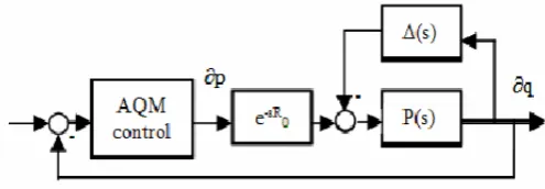
Fig. 1. Block diagram of AQM as a feedback control system
A.Linearized model
Although an AQM router is clearly a non-linear system, in order to analyze certain required properties and design linear controllers, a linearized model is used. To linearize (1) and (2), it is assumed that the number of active TCP sessions and the link capacity are constant, i.e., NTCP(t)=NTCP=N and C(t)=C.
As described in [5] and [9], the dependence of the time delay argument t−R on the queue length q is ignored, so it is assumed to be fixed at t−R0. This is a big assumption and
round-trip time is dominated by the propagation delay. When the model is linearized, the same supposition is made. It cannot be denied that calculations are significantly simplified, so further research in the matter would be advisable.
Then, the local linearization of (1) and (2) around the operating point
q0,p0,W0
results in the followingequations:
) ( 1 ) ( ) ( 1 2 1 2 1 0 0 0 0 2 2 0 0 0 2 0 0 0 0 0 0 t q R t W R N t q R t p R T N C R T T R R t q t q C R R T R t W t W C T R N t W p q p p q (3)where Tq0 R0Tp, W(t)WW0 and p pp0
represent the perturbed variables. Taking (W,q) as the state and p as the input, the operating point
q0,p0,W0
is definedby W 0 and q0, that is,
00 3 2 0 0 0 2 0 p T R N T R R W W p p , 0 0
0 q N W
q . (4) Equation (3) can be further simplified by separating the low frequency (‘nominal’) behaviour P(s) of the window dynamic from the high frequency behaviour ∆(s), which is considered parasitic. Taking (4) as the starting point and following steps similar to those in [5], we can obtain the feedback control system in Fig. 1 and equations (5) to (7) for TCPW/AQM ([14]).
The action implemented by an AQM control law is to mark packets, with a discard probability p(t), as a function of the measured queue length q(t). Thus, the larger the queue, the greater the discard probability becomes.
p p p T R T R R C N s R C N R C s R T N C s P 0 0 3 0 2 0 0 2 0 2 2 2 1 (5)
1 1
1 0
0
sR e C R
s
(6)
[image:3.595.320.548.68.107.2]Where: 0 20 2 1 R T N R C p (7)
Fig. 2. Block diagram of the AQM feedback control system
IV. APPROXIMATINGTHESYSTEMDELAY This section briefly describes how the system delay can be approximated when working with a transfer function in the Laplace transform domain, so that the transfer function can be expressed as a quotient of rational polynomials.
Initially, the delay term sT
e
can be approximated by its Maclaurin series (i.e., its Taylor series centred in s=0). The main characteristic is that the numerator of the rational approximation is constant, but as there are no dynamics for this term, the results are worse than with other approximations such as Padé.The Padé approximation is the most frequent approach for obtaining a transfer function estimate of the system delay: the exponential function is first expanded into a Maclaurin series and then approximated by a rational function. The higher the order of the series is, the better but more complex the approximation will be.
As [15] emphasizes, most books and papers work with an approximation having the same numerator and denominator degree, so the step response of the system when using this approximation has a discontinuity at t=0. Moreover, the numerator of the Padé approximation has zeros at the right hand side of the continuous plane. These non-minimum phase zeros can be a problem when tuning the controller, as they cannot be cancelled and introduce dynamics that are not present in the original system.
To solve the jump at the origin, [15] proposed a modified Padé approximation such that the degree of the numerator is lower than the degree of the denominator. This approach has an important consequence: if the first order approximation is chosen, then there are no minimum-phase zeros. The classical Padé approximation is shown in (8) and the modified one in (9).
Moreover, if the first order approximation is considered (8):
Ts
Ts
e
Ts
2
2
(8)Ts
e
Ts
1
1
(9) The paper will show controllers tuned using these two approaches to deal with the system dead-time.V. POLEPLACEMENTCONTROLLER
Pole placement is a technique for designing controllers that can be applied to stable and unstable systems, there are no restrictions upon the model zeros (stable or unstable). The most important characteristic is that the closed loop transfer function can be chosen to obtain a fast response and a good control signal.
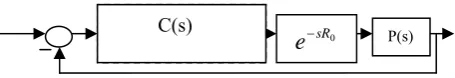
CPID K1
e
sR0 P(s)There are several approaches that can be followed to obtain a pole placement controller. This paper presents the simplest one. First, the method will be described and then applied to the AQM congestion control problem in a network with wireless links.
Let us have:
G(s): transfer function of the plant to be controlled. C(s): controller to be designed.
H(s): desired closed loop transfer function, such that the unstable open loop poles and zeros are included and the characteristic equation includes the desired behaviour in terms of velocity of response and error.
Then:
s
G
s
C
s
G
s
C
s
H
1
(10)and, as we choose H(s), the controller will be:
s
H
s
H
s
G
s
C
1
1
(11) The degree of H(s) must be greater than or equal to the degree of G(s). In general, the greater the degree of H(s), the better the control signal will be.
The previous section presented the transfer function of TCPW and how the delay affected the system. Now, the pole placement controller will be derived, depending on the delay approximation.
The three different controllers will have zero steady error when an input step is applied.
A.Pole placement controller without delay
If no delay is taken into account, the controller will be:
s
H
s
H
s
P
s
C
wd wd wd
1
1
(12) where P(s) is given by (5) and Hwd(s) will be chosen
depending on the network parameters.
B.Pole placement controller with classical Padé approximation
If no delay is taken into account, the controller will be:
s
H
s
H
s
P
s
D
s
C
d D
d
1
1
(13) where P(s) is given by (5), D(s) is given by (8) such that T=R0 and Hd(s) must explicitly consider the non-minimum
phase zero of D(s) and it will also depend on the network parameters.
C.Pole placement controller with alternative Padé approximation
If no delay is taken into account, the controller will be:
s
H
s
H
s
P
s
D
s
C
ad ad a
ad
1
1
(14) where P(s) is given by (5), Da(s) is given by (9) such that
T=R0 and only Had(s) will depend on the network
parameters, because there are non-minimum phase zeros. In the next section, the network parameters are defined. The linear and non-linear simulations will show the goodness of the method depending on the delay approximation.
VI. SIMULATIONS A.Tuning the Controller
The basic network topology used as an example to test the controller is depicted in Fig. 3. It is a typical single bottleneck topology. The link capacity (C) is kept constant in all experiments it is set to. The number of users (N) is set to 70 and the round trip time (R0) to 1.1 seconds. These
[image:4.595.307.546.179.311.2]settings reflect a high number of users, quite a large delay and a not very fast link.
Fig. 3. Dumbbell topology
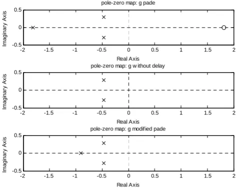
Fig. 4 shows the open loop poles of the system without the delay, the open loop poles when a Padé approximation is considered, and the open loop poles with the modified Padé approach. The pair of complex conjugate poles are the system’s poles. The right hand side zero is due to the classic Padé formula.
-2 -1.5 -1 -0.5 0 0.5 1 1.5 2 -0.5
0 0.5
pole-zero map: g pade
Real Axis
Im
agi
nar
y
A
x
is
-2 -1.5 -1 -0.5 0 0.5 1 1.5 2 -0.5
0 0.5
pole-zero map: g w ithout delay
Real Axis
Im
agi
nar
y
A
x
is
-2 -1.5 -1 -0.5 0 0.5 1 1.5 2 -0.5
0 0.5
pole-zero map: g modif ied pade
Real Axis
Im
agi
nar
y
A
x
[image:4.595.306.543.415.607.2]is
Fig. 4. Open loop poles and zeros
0 2 4 6 8 10 12 -30
-20 -10 0
Open loop step response: g pade
Time (sec)
A
m
pl
itude
0 2 4 6 8 10 12
-30 -20 -10 0
Open loop step response: g w ithout delay
Time (sec)
A
m
pl
itude
0 2 4 6 8 10 12
-30 -20 -10 0
Open loop step response: g modified pade
Time (sec)
A
m
pl
[image:5.595.50.286.56.259.2]itude
Fig. 5. Step responses
First, the closed loop transfer function must be chosen. As we have three different situations, there will be three different closed loop transfer functions, although there are common settings for the three cases. Let us choose a settling time of 6 seconds and a damping ratio of 0.8 (basic transfer function (15)):
7 . 0 34 . 1 7 . 02 2 2
2 2 s s w s w s w s H n n n
(15)
This transfer function is a bit faster than the original system. It is also important to note that the closed loop error will be zero: an integrator is implicitly included in the design.
When no delay is considered, the closed loop transfer function of the system will be given by (16) and the controller by (17).
16
.
3
75
.
6
88
.
5
16
.
3
1
22
.
0
1
23
s
s
s
s
s
H
s
H
wd (16)
7 . 6 9 . 5 98 . 0 05 . 3 24 . 3 10 2 2 4 s s s s s sCwd (17)
In this case, the degree of the closed loop transfer function is set to 3 to improve the control signal. Theoretically, a degree of 2 is enough.
If the Padé approximation is used, the closed transfer function is given by (18) and the controller by (19). The right-hand-side zero has to be included in Hd(s). It cannot be
cancelled. The third pole is placed such that it cancels the delay pole and the fourth pole is located a bit farther to improve the control signal and not compromise the closed-loop response.
4 . 5 44 . 15 44 . 17 7 . 7 4 . 5 16 . 3 1 22 . 0 1 1 55 . 0 1 2 34
s s s s s s s H s Hd (18)
s s s s s s s s Cd 6 . 18 44 . 17 7 . 7 8 . 1 55 . 6 9 . 8 2 . 3 10 2 3 2 3 4 (19)
If the alternative Padé approximation is used, the closed transfer function is given by (20) and the controller by (21). Again, the third pole cancels the delay pole and the fourth pole improves the control signal.
87 . 2 3 . 9 1 . 12 8 . 6 87 . 2 1 22 . 0 1 1 1 . 1 1 2 34
s s s s s s s H s Hd (20)
s s s s s s s s Cd 3 . 9 1 . 12 8 . 6 9 . 0 7 . 3 6 2 . 3 10 2 3 2 3 4 [image:5.595.306.547.142.234.2] (21)
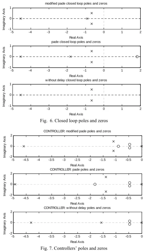
Fig. 6 shows the closed loop poles and zeros for the three cases under study and Fig. 7 depicts the poles and zeros of the controllers.
B.Linear Simulations
-5 -4 -3 -2 -1 0 1 2 -1
0 1
pade closed loop poles and zeros
Real Axis Imag inar y A x is
-5 -4 -3 -2 -1 0 1 2 -1
0 1
modified pade closed loop poles and zeros
Real Axis Imag inar y A x is
-5 -4 -3 -2 -1 0 1 2 -1
0 1
w ithout delay closed loop poles and zeros
Real Axis Imag inar y A x is
Fig. 6. Closed loop poles and zeros
-5 -4.5 -4 -3.5 -3 -2.5 -2 -1.5 -1 -0.5 0 -2
0 2
CONTROLLER: pade poles and zeros
Real Axis Imag inar y A x is
-5 -4.5 -4 -3.5 -3 -2.5 -2 -1.5 -1 -0.5 0 -2
0 2
CONTROLLER: modif ied pade poles and zeros
Real Axis Im agi na ry A x is
-5 -4.5 -4 -3.5 -3 -2.5 -2 -1.5 -1 -0.5 0 -2
0 2
CONTROLLER: w ithout delay poles and zeros
Real Axis Im agi n ar y A x is
Fig. 7. Controllers’ poles and zeros
[image:5.595.302.545.306.729.2] [image:5.595.79.278.473.569.2]the transfer function of the plant and the delay approximated with Padé works well, and that the transfer function and the alternative delay approximation and the corresponding controller also work well.
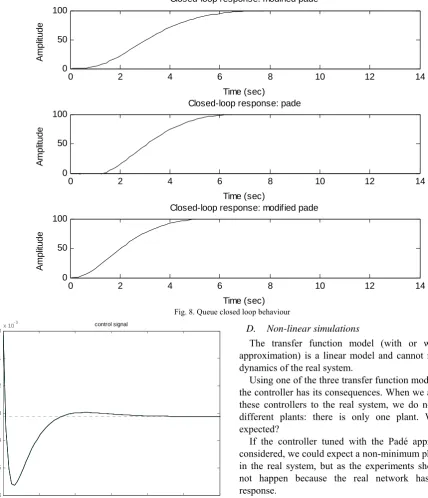
The queue reference changes in 100 packets. Fig. 8 shows the three step responses. It can be seen how, in the
three cases, the systems behave as they should: the
non-delay transfer function of the plant responds without non-delay, the step response of the transfer function of the plant in conjunction with the Padé approximation presents a non-minimum phase behaviour, and the modified Padé approach
step response shows the delay but NO minimum phase behaviour. As shown in Fig. 9, the control signal in the three cases have no differences. They are all the same.
0 2 4 6 8 10 12 14
0 50 100
Closed-loop response: pade
Time (sec)
A
m
pl
itude
0 2 4 6 8 10 12 14
0 50 100
Closed-loop response: modified pade
Time (sec)
A
m
pl
itude
0 2 4 6 8 10 12 14
0 50 100
Closed-loop response: modified pade
Time (sec)
A
m
pl
[image:6.595.65.494.145.644.2]itude
Fig. 8. Queue closed loop behaviour
0 2 4 6 8 10 12
-6 -5 -4 -3 -2 -1
0x 10
-3 control signal
Time (sec)
A
m
pl
itude
Fig. 9. Control signal
D. Non-linear simulations
The transfer function model (with or without delay approximation) is a linear model and cannot reflect all the dynamics of the real system.
Using one of the three transfer function models for tuning the controller has its consequences. When we apply/migrate these controllers to the real system, we do not have three different plants: there is only one plant. What can be expected?
If the controller tuned with the Padé approximation is considered, we could expect a non-minimum phase response in the real system, but as the experiments show, this does not happen because the real network has no inverse response.
0 10 20 30 40 50 60 70 80 90 100 200
300 400
QUEUE: modified Pade
0 10 20 30 40 50 60 70 80 90 100
200 300 400
QUEUE: Pade
0 10 20 30 40 50 60 70 80 90 100
200 300 400
QUEUE: without delay
[image:7.595.140.461.56.315.2]
Fig. 10. Queue evolution: three different controllers and the real plant
0 10 20 30 40 50 60 70 80 90 10
0 5
x 10-3 PROBABILITY: modified Pade
0 10 20 30 40 50 60 70 80 90 10
0 5
x 10-3 PROBABILITY: Pade
0 10 20 30 40 50 60 70 80 90 10
0 5
x 10-3 PROBABILITY: without delay
Fig. 11. Probability
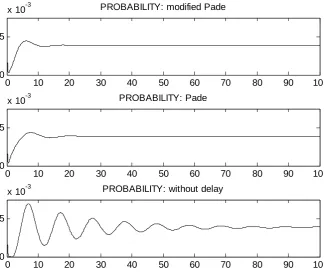
The experiment applies the same change to the reference: change from 100 to 200 packets.
In Fig. 10, the queue evolution of the non-linear model of the network working with TCPW is shown. The queue evolution, when the controller is the one tuned, considering no delay in the plant is bad. The same can be said about the discarding probability (Fig. 11). Moreover, if we compare the results of the linear and the non-linear simulation, there are many differences. We can conclude that the controller was validated using the transfer function and no delay and this does not correspond to reality.
The Padé controller and the modified Padé controller present a very good behaviour. But it should be noted that when the controllers were validated using the transfer function model and the corresponding delay approximation, the Padé one exhibited a non-minimum phase behaviour that does not appear in the non-linear study. The reason is very simple: the real system is minimum phase.
[image:7.595.138.463.347.626.2]response in the linear case. Fig. 14 shows that the controller tuned considering the system as delay free is not acceptable
VII. CONCLUSIONS
The paper has presented a comparison between three different pole placement controllers. Results show that this technique can give good results for dealing with the congestion control problem.
If the controller is tuned without considering the plant delay, the results will be bad. Networks have delays and they should be taken into account in the controller design.
The other two controllers were designed using a rational approximation for the delay. When the classic approach was followed, the linear queue evolution was good, but exhibited an inverse response that the real network does not have. The modified delay approach solved this problem. These results are valid when the first order approximation is used.
Future work involves including uncertainties in the model description and more complex topologies.
0 5 10 15 20 25 30 35 40
200 220 240 260 280 300 320 340
non-linear linear
Fig.. 12. QUEUE, comparison between the non-linear model and the linear-model with the modified Padé approach
0 5 10 15 20 25 30 35 40
180 200 220 240 260 280 300 320 340
non-linear linear
Fig.. 13. QUEUE, comparison between the non-linear model and the linear-model with the classic Padé approach
.
ACKNOWLEDGMENT
The author would like to thank Prof. F. Tadeo for so many fruitful discussions.
0 5 10 15 20 25 30 35 40
200 220 240 260 280 300 320 340 360 380 400
non-linear linear
Fig.. 14. QUEUE, comparison between the non-linear model and the linear-model with no delay approach
REFERENCES
[1] T. Azuma, T. Fujita, and M. Fujita, “Congestion control for TCP/AQM networks using State Predictive Control,” Electrical Engineering in Japan, vol. 156, pp. 1491-1496, 2006.
[2] Deng, X., S. Yi, G. Kesidis. C.R. Das, “A control theoretic approach for designing adaptive AQM schemes” in Proc. GLOBECOM’03, San Francisco, 2003, pp. 2947 – 2951
[3] V. Jacobson, “Congestion avoidance and control” in Proc. ACM SIGCOMM’88, Stanford, 1988.
[4] S. Ryu,, C. Rump and C. Qiao, “Advances in Active Queue Management (AQM) based TCP congestion control.,” Telecommunication Systems, vol. 25, pp. 317-351, 2004.
[5] C.V. Hollot, V. Misra, D. Towsley and W. Gong “Analysis and Design of Controllers for AQM Routers Supporting TCP flows,” IEEE Transactions on Automatic Control, vol. 47, pp. 945-959, 2002 [6] P.H. Lewis and C. Yang, Basic Control Systems Engineering.
Prentice-Hall, New Jersey, USA , 1997.
[7] Q. Chen, and O.W.W. Yang, “On designing self-tuning controllers for AQM routers supporting TCP flows based on pole placement,” IEEE Journal on Selected Areas in Communications, vol. 22, pp. 1965-1974, 2006.
[8] J. Chen, F. Paganini, M.Y. Sanadidi, R. Wang and M. Gerla, “Fluid-flow analysis of TCP Westwood with RED,” Computer Networks, vol. 50, pp. 132-1326, 2006.
[9] M. di Bernardo, L. A. Grieco, S. Manfredi, and S. Mascolo, “Design of robust AQM controllers for improved TCP Westwood congestion control” in Proc. of the 16th International Symposium on
Mathematical Theory of Networks and Systems (MTNS 2004), Katholieke Universiteit Leuven, Belgium, July, 2004.
[10] S. Mascolo, C. Casetti, M. Gerla, M.Y. Sanadidi and R. Wang, “TCP Westwood: bandwidth estimation for enhanced transport over wireless links,” in Proc. of Mobicom, Rome, Italy, 2001.
[11] R. Wang, M. Valla, M.Y. Sanadidi, B. Ng and M. Gerla, “Efficiency/friendliness tradeoffs in TCP Westwood,” in Proc. IEEE Symposium on Computers and Communications, Taormina, Italy, July 2002.
[12] R. Wang, M. Valla, M.Y. Sanadidi and M. Gerla, “Adaptive bandwidth share estimation in TCP Westwood,” in Proc. of IEE Globecom, Taipei, 2002.
[13] C.V. Hollot, and Y. Chait (2001). Nonlinear stability analysis for a class of TCP/AQM networks”. In Proceedings of the 40th IEEE
Conference on Decision and Control, Orlando, USA
[14] Alvarez, T. (2012). Designing and Analysing Controllers for AQM routers working with TCP Westwood protocol (unpublished). [15] Vajta, M. Some remarks on Padé-Approximations. Proceedings of 3rd