Filter Design and Measurement Lab 08

ECE 300 Signals and Systems Fall 2007

Filter Design and Measurement

Lab 08

by Bruce A. Black, Robert Throne, and Mario Simoni

Objectives

In this lab we will examine filters in different ways. We will first investigate three different kinds of lowpass filters and the properties they possess. These filters illustrate the types of trade-offs we must make when designing a system. We will then experimentally measure the magnitude of the frequency response of a fifth order Butterworth filter and compare this with the predicted response. Finally we will use a filter to measure the relevant “bandwidth” of a signal and look at the effects of filtering on a “real-world” signal.

Equipment

Agilent Function Generator Digital Oscilloscope

Orange Butterworth Filter

BNC T-connector 50 Ω termination Floppy disk

Background

A periodic signal can be represented by the complex exponential form of the Fourier series. When a periodic signal is applied to the input of a filter, each of the harmonic components of the input signal experiences an amplitude and phase change caused by the filter. At the filter output the harmonic components add together to produce the output waveform. The amplitude and phase changes experienced by each of the input components combine to make the output signal different from the input signal in a predictable way. This difference between the input and output waveform is called distortion.

Stated mathematically, suppose x(t) is a periodic input signal with period T0, H(ω) is the frequency response of the filter (i.e. the Fourier transform of its input response h(t)), and y(t) is the filter output. Then the input x(t) can be written

( )

0 0

, where 2

jk t k k

x t a e ω ω π

∞

=−∞

=

∑

As the input signal passes through the filter, the input coefficients ak become altered by the filter to

become the output coefficients bk, where

(

)

k k

b =H kω a . The output y(t) is then given by

( )

(

)

0

jk t jk t

k k

k k

y t b e ω H kω a e ω

∞ ∞

=−∞ =−∞

In practice there is not usually an infinite number of components to be added to produce either x(t) or y(t); only components with significant amplitudes need to be included.

Pre-Lab

Part 1: Filtering Periodic Signals

This is a continuation of the work you did in Lab 6. Now we are going to concentrate a bit more on the filters and examine some trade-offs between different common types of lowpass filters. Much of what follows is the same as for Lab 6, but there are a few changes at the end when we use different types of filters.

a) Use your code from Lab 6 to determine the Complex Fourier series representation using 20 terms of the following periodic function (defined over one period).

0 2

1 1 2

( )

3 2 3

0 3 4

t t x t t t 1

− ≤ < − ⎧

⎪ _{− ≤ <}

⎪

= ⎨ _{≤ <}

⎪

⎪ _{≤ <}

⎩

b) For the majority of the filters it uses, Matlab assumes filter has the form

1 2

1 2 1

1 2

1 2 1

( )

N N

N N

N N

N N

b s b s b s b s b H s

a s a s a s a s a

− − − − 0 0 + + + + + = + + + + + " "

Hence, in order to represent any filter, Matlab just uses an array for the b coefficients and an array for the a coefficients. For example, we might have two variables (arrays) B and A to store the coefficients. These variables would be

[

]

[

]

B b b b

A a a

=

= a

Let’s assume we want to use a 10th order Butterworth lowpass filter with a frequency cutoff of 20ω₀. Use the help command to look up the Matlab function butter. You should return the coefficients in two arrays, i.e. your command should be [B,A] = butter(…..); Note that we are constructing an analog filter here, so read all of the description for the butter command.

c) We now again need to find the variable H0 = H(0) the variable (array)

[

]

H = H jω H j ω H jNω₀ . To find H(0) we use the fact that

0 0 (0) b H a =

H0 = B(end)/A(end);

Where end tells Matlab to get the last element of the array. The command freqs will be helpful for finding the variable (array) H.

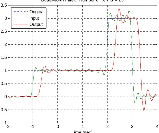
d) Plot the Fourier series representation for both the input signal x t( ) and the output signal on the same graph for N=25 terms, using different line types and a legend. The title of your graph should indicate that you are using a Butterworth filter. If you have done everything correctly your graph should look like that in Figure 1. Print out this graph and attach it to the worksheet at the end of this lab.

( )

y t

-2 -1 0 1 2 3 4

-1 -0.5 0 0.5 1 1.5 2 2.5 3 3.5

Time (sec)

Butterworth Filter, Number of Terms = 25

Original Input Output

Figure 1. Input and Fourier series representation of the input and output using a 10th order Butterworth filter.

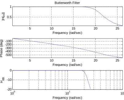
It will be useful to look at a frequency response plot of the filter you are using. You will need to make three plots on one page using the subplot command. Type orient tall before any of the plotting so you can use more of the page.

e) The first plot is the magnitude of the transfer function as a function of frequency. You will need to use the abs command. You should also put a grid on your figure.

f) The second plot is the phase of the transfer function (in degrees) as a function of frequency. In order to see the phenomena we want to see use the sequence of commands unwrap(angle(H))*180/pi. The most important command here is unwrap, which allows angles of more than 180 degrees

Be sure to include the type of filter you are using in your title. If you have done everything correctly, you should get a plot like that shown in Figure 2. Print out this graph and attach it to the worksheet at the end of the lab.

5 10 15 20 25

0.5 1

Frequency (rad/sec)

|H(

ω

)|

Butterworth Filter

5 10 15 20 25

-500 -400 -300 -200 -100

Frequency (rad/sec)

P

h

as

e

(

d

eg

)

100 101 102

-20 -10 0

Frequency (rad/sec) H dB

Figure 2. Frequency response of the 10th order Butterworth filter.

h) If the phase of the filter is exactly linear then we should have the relationship

( sec)

slope of filter in time delay

− =

Using a straight edge (or ruler), draw a line on your graph between the initial point on the phase graph and the value of the phase at about 20ω0. Estimate the delay between the input and output signal (use

Matlab to zoom in on the signal and measure this accurately, don’t just eyeball it!) and compare this to the predicted delay. Fill in the table on the worksheet.

approximately 20ω_o. For this use multiples of ω_o, such as 30ω_o, 40ω_o, etc. Be sure to print out both graphs.

j) Repeat parts b-h using a Cheyshev filter (use the command cheby1 and the defaults if you don’t know what values to use). Be sure to print out both graphs.

k) In the Chebyshev filter, try varying the R parameter from 0.5 (the default) to 2.0. What happens to the filter?

Part 2: Measuring the Frequency Response

a) Obtain an orange filter from your instructor.

b) Set the function generator to output a 1V peak-to-peak sine wave. Be sure to properly account for the necessary 50 Ω load.

c) Set the frequency of the signal generator to 100 Hz, and adjust the amplitude of the sine wave so the output of the signal (after passing through the orange filter) is measured as 1V peak peak-to-peak on the oscilloscope.

d) Measure and record the frequency and the output amplitude (measured on the scope) as the frequency is varied so you can fill in the table on the worksheet at the end of the lab. Near the cutoff frequency of the filter, f_c, measure the amplitudes at frequencies f_c−200, f_c−100, , and

Hz .

100 c

f + 200

c

f +

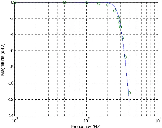
e) The orange filter is a fifth order filter. Using your estimated cutoff frequency, generate the

corresponding Butterworth filter in Matlab using the butter command. We are constructing an analog filter, and be sure your cutoff frequency is in the correct units.

102 103 104 -14

-12 -10 -8 -6 -4 -2 0

Frequency (Hz)

M

a

gn

it

ud

e (

dB

V

)

Figure 3: Predicted and measured frequency response.

Part 3: Measuring the Bandwidth of a Signal

Even though the Fourier Transform of a signal can take up the entire spectrum to infinite frequency, you don’t necessarily need the entire spectrum to get the relevant “information” from a signal. In this part of the lab, you will be applying filters to the ECE300 welcome message that you heard on the first day of class. The goal will be to find the minimum bandwidth that includes all of the necessary

“information”, and then relate this information to the power spectrum of the signal.

When MATLAB is used to filter a signal, everything must be done with discrete-time signal

processing tools because it is being implemented on a computer. You will learn more about these tools in ECE380. For this lab the signal has been sampled at a sufficiently high frequency to approximate the continuous time equivalent. The only difference as far as you are concerned is how the filter cutoff frequency is defined. Instead of an absolute frequency, it must be normalized to half the sampling frequency. This has already been accounted for in the supplied script file so that you can still specify the absolute frequency in units of Hz.

a) Copy the files welcomeMsg.mat and lab8msg.m to your working directory for lab8. Look over the script file and make sure you understand what it is doing. You will need to add the appropriate axis labels and titles to all of your plots before printing them out.

b) Start by using a lowpass filter with a cutoff frequency of 50 Hz. Look at the spectrum and the time waveform and listen to the message. Describe what happened to the signal in the time and frequency domain on the lab worksheet. Also explain why the speaker doesn’t produce any sound for the filtered signal.

figures that illustrate the time and frequency representation of the signal. When you find the final cutoff frequency, record it on the lab worksheet and print out the two figures to turn in with your lab.

d) Now switch to a highpass filter and start with a cutoff frequency of 4kHz. Look at the spectrum and the time waveform and listen to the message. Describe what happened to the signal in the time and frequency domain on the lab worksheet. Also describe the sound that you hear from the speaker.

e) Decrease the cutoff frequency of the highpass filter in regular increments until you don’t hear much difference between the “words” of the original and filtered messages. For each increment, observe the figures that illustrate the time and frequency representation of the signal. When you find the final cutoff frequency, record it on the lab worksheet and print out the two figures to turn in with your lab.

Lab 08

Instructor Verification Sheet

Names___________________________Date:___________

At the end of this lab you should have attached the following plots:

• Two plots for the Butterworth filter (input/output and transfer function characteristics)

• Two plots for the Bessel filter

• Two plots for the Chebyshev filter

• One plot for matching determining the frequency response of the filter

• The six plots from Part 3 (lowpass time/ freq, highpass time/freq, bandpass time/freq)

Part 1: Measurements of Different Filters

Part 2: Measuring the Frequency Response of a Real Filter

Filter Type

Predicted Delay

(-slope of filter)

Measured Delay (time domain)

10th order Butterworth 10th order Bessel 10th order Chebyshev

Frequency (Hz) 100 500 1000 1500 2000 2500 3000 3500 4000 Amplitude

Frequency (Hz) f_c−200

100

c

f−

100 c

f −

c

f

? c

f = f_c+100 200f_c+

Amplitude

Part 3: Measuring the Bandwidth of a signal

Lowpass filter cutoff frequency Highpass filter cutoff frequency

Question 2: From Part 1, which filter has the flattest magnitude response over the passband? This filter will have the smallest magnitude distortion.

Question 3: From Part 1, which filter has the steepest rolloff after the cutoff frequency ?

Question 4: From Part 1, what is the effect of varying R in the Chebyshev filter?

Question 5: What happened to the WelcomeMsg signal in the time and frequency domain when the lowpass filter cutoff frequency was 50 Hz?

Question 6: What happened to the WelcomeMsg signal in the time and frequency domain when the highpass filter cutoff frequency was 4 kHz?

Question 7: What relationship do you notice between the bandwidth of the bandpass filter and the spectrum of the original WelcomeMsg signal?