Numerical Method for Solving Electromagnetic Scattering Problem by Many Small Impedance Bodies

http://www.scirp.org/journal/ajcm ISSN Online: 2161-1211

ISSN Print: 2161-1203

DOI: 10.4236/ajcm.2017.74031 Dec. 14, 2017 435 American Journal of Computational Mathematics

Numerical Method for Solving Electromagnetic

Scattering Problem by Many Small

Impedance Bodies

Nhan T. Tran

Department of Mathematics, Kansas State University, Manhattan, USA

Abstract

In this paper, we study electromagnetic (EM) wave scattering problem by many small impedance bodies. A numerical method for solving this problem is presented. The problem is solved under the physical assumptions ka1, where a is the characteristic size of the bodies and k is the wave number. This problem is solved asymptotically and numerical experiments are provided to illustrate the idea of the method. Error estimate for the asymptotic solution is also discussed.

Keywords

Electromagnetic Scattering, Integral Equation, Boundary Impedance, Many-Body Scattering, EM Waves

1. Introduction

Electromagnetic scattering is the effect caused by EM waves such as light or ra-dio waves hitting an object. The waves will then be scattered and the scattered field contains useful information about the object, see [1] [2][3]. Electromag-netic scattering happens in many situations, for example, sun light scattered by atmosphere, radio waves scattered by buildings or planes, and so on. The study of EM wave scattering is of great interest and importance since it helps advance many different fields ranging from Medical Technology to Computer Engineer-ing, Geophysics, Photonics, and Military Technology, see [2][4]. Unfortunately, most wave equations cannot be solved analytically to get an exact solution. Therefore, numerical methods are sought to approximate the solution asymp-totically. Unlike solving scalar wave scattering problem [5][6], solving EM wave scattering is much more complicated and computationally expensive due to the

How to cite this paper: Tran, N.T. (2017) Numerical Method for Solving Elec-tromagnetic Scattering Problem by Many Small Impedance Bodies. American Journal of Computational Mathematics, 7, 435-443.

https://doi.org/10.4236/ajcm.2017.74031

Received: October 26, 2017 Accepted: December 11, 2017 Published: December 14, 2017

Copyright © 2017 by author and Scientific Research Publishing Inc. This work is licensed under the Creative Commons Attribution International License (CC BY 4.0).

http://creativecommons.org/licenses/by/4.0/

DOI: 10.4236/ajcm.2017.74031 436 American Journal of Computational Mathematics vector nature of EM waves.

In [7] and [8], a theory for solving electromagnetic wave scattering problem by many small perfectly conducting and impedance bodies was developed. In [9] [10], numerical methods for solving EM wave scattering by one and many small perfectly conducting bodies are presented. In this paper, we focus on EM wave scattering by many small impedance bodies. A numerical method for solving this problem, based on the above theory, is described and tested. The problem is solved under the assumptions that the characteristic size a of the bodies is much smaller than the distance d between neighboring bodies,

2 3

d O a

κ −

 

=  

  where

[

0,1

)

κ

∈ _{, and this distance d is much less than the wave length}

λ

_, ka1 where k is the wave number. The distribution of these small bodies is assumed to follow this law

( )

2

( )

( )

1

d 1 1 , 0,

N x x o a

a −κ ∆

∆ =

∫

_ + _ →

 (1)

in which ∆ is an arbitrary open subset of the domain Ω that contains all the small bodies, 

( )

∆ is the number of the small bodies in ∆, and N is the distribution function of the bodies

( )

0,

( )

( )

.

N x ≥ N x ∈ ΩC (2)

The boundary impedance of the bodies is of the form

ζ

=ha−κ, where h is a

continuous function such that Imh≥0, and

κ

∈

[

0,1

)

. The function h and constant κ can be chosen as desired.

To make the paper self-contained, the theory of EM wave scattering by one and many small impedance bodies is given in Sections 2 and 3. In Section 4, a numerical method for solving the EM scattering problem is presented. The solution of this problem is computed asymptotically and error analysis of the asymptotic solutions is also provided.

2. Electromagnetic Wave Scattering by One Small

Impedance Body

Let D be a bounded domain of one small body, a be its radius, and S be its

smooth boundary, 1,

(

]

, 0,1

S∈C γ γ∈ . Assume that the dielectric permittivity 

and magnetic permittivity

µ

_{are constants. Let E and H denote the electric}

field and magnetic field, respectively. E0 is the incident field and vE is the scattered field. The electromagnetic wave scattering by one small impedance body problem can be stated as follows

3

, in : \ ,

E i

ωµ

H D′ D

∇ × = =_{ (3)}

, in ,

H iω E D′

∇ × = −  (4)

[

]

[

]

, , , , Re 0,

N E N =

ζ

N H

ζ

≥

 

  (5)

0 E,

E=E +v (6)

2

0 e , 0, ,

ik x

DOI: 10.4236/ajcm.2017.74031 437 American Journal of Computational Mathematics 1

, : ,

E E

v

ikv o r x

r r

∂ _{− =}   _{= → ∞}

 

∂   (8)

where

ω

>0 is the frequency, k=2π λ ω µ=  is the wave number, ka1,

λ

_{is the wave length,}

ζ

is the boundary impedance of the body, and α is a unit vector that indicates the direction of the incident wave E0. This incident

wave satisfies the relation ∇ ⋅E0=0. The scattered field vE satisfies the radiation condition (8). Here, N is the outward pointing unit normal to the surface S.

It is known from [8] that problem (3)-(8) has a unique solution and its solution is of the form

( )

0

( )

( ) ( )

( )

e

, d , , : ,

4π ik x t

S

E x E x g x t J t t g x t

x t

−

= + ∇ × =

−

∫

(9)

where E0 is the incident plane wave defined in (7) and J is an unknown

pseudovector. J is assumed to be tangential to S and can be found from the impedance boundary condition (5). Here E is a vector in 3 _and

E

∇ × is a pseudovector.

Once we have E, from (3) H can be found by the formula

,

E H

iωµ

∇ ×

= ₍₁₀₎

The asymptotic formula of E when the radius a of the body D tends to zero is

( )

0

( )

x

(

, 1

)

, ,

E x =E x + ∇_ g x x Q_ (11)

where x−x1 a, and the point x1 is an arbitrary point inside the small body

D, see [8]. So, instead of finding J to get E, we can just find one pseudovector Q

( )

d . S

Q=

∫

J t t (12)

The analytical formula for Q is derived in [8] which can be summed up in the following theorem.

Theorem 1. One has

0

S

Q E

i

ζ τ ωµ

= − ∇ × (13)

where

( )

( ) ( )

3

1

: , _jm : _{j m} d ,

S

I b b b N s N s s

S

τ = − = =

∫

₍₁₄₎

and S is the surface area of S.

Here, 1≤ j m, ≤3 correspond to x y, , and z coordinates in 3, I₃ is a 3 ×

3 identity matrix, and Nj,1≤ ≤j 3 is the j-th component of the outer unit normal vector to the surface S.

3. Electromagnetic Wave Scattering by Many Small

Impedance Bodies

DOI: 10.4236/ajcm.2017.74031 438 American Journal of Computational Mathematics m

S are their corresponding smooth boundaries. Let

1

: M _m

m

D =



₌D ⊂ Ω and D'

be the complement of D in 3_{. We assume that} 1,

(

]

1 , 0,1

M m m

S=



₌S ∈C γ γ∈ .

We also assume that the dielectric permittivity  and magnetic permittivity

µ

are constants. Let E and H denote the electric field and magnetic field, respectively. E0 is the incident field and v is the scattered field. The

electromagnetic wave scattering by many small impedance bodies problem involves solving the following system

3

1

, in : \ , : ,

M

m m

E iωµH D D D D

= ′

∇ × = = =



(15)

, in ,

H iω E D′

∇ × = −  (16)

[

]

[

]

, , m , , on m, 1 ,

N E N =ζ N H S ≤m≤M

 

  (17)

0 ,

E=E +v (18)

2

0 e , 0, .

ik x

E = α⋅ ⋅ =

α

α

∈S (19)

where v satisfies the radiation condition (8),

ω

>0 is the frequency, k=2π λ

is the wave number, ka1, : 1max diam

2 m m

a = D , α is a unit vector that

indicates the direction of the incident wave E0, and ζm is the boundary impedance of the body Dm. These ζm’s are given by the following formula

( )

, 0 1, , 1 ,

m

m m m

h x

x D m M

aκ

ζ

= ≤ <

κ

∈ ≤ ≤ (20)

where h x

( )

is a continuous function in a bounded domain Ω,

( )

Reh x 0, Imε σ 0, ω

≥ = ≥ ₍₂₁₎

3

0, 0 in : \ .

ε ε

=

µ µ

= Ω =′ _ Ω ₍₂₂₎

The distribution of small bodies Dm , 1≤ ≤m M , in Ω satisfies the following assumption

( )

2

( )

( )

1

d 1 1 , 0,

N x x o a

a −κ ∆

∆ =

∫

_ + _ →

 (23)

where 

( )

∆ is the number of small bodies in ∆, ∆ is an arbitrary open subset of Ω,

( )

0,

( )

( )

N x ≥ N x ∈ ΩC (24)

and

κ

∈

[

0,1

)

is the parameter from (20). From (15) and (16) we have

2 2 2

, ,

E k E k

ω µ

∇ × ∇ × = =  (25)

if

µ

=const. Once we have E, then H can be found from this relation

.

E H

iωµ

∇ ×

= ₍₂₆₎

DOI: 10.4236/ajcm.2017.74031 439 American Journal of Computational Mathematics assumptions (21), the problem (15)-(18) has a unique solution and its solution is of the form

( )

0

( )

( ) ( )

1

, d .

m M

m S

m

E x E x g x t J t t

=

= +

∑

∇ ×

∫

(27)

where

( )

: d .

m m _S m

Q =

∫

J t t (28)

When a→0, the asymptotic solution for the electric field is given by

( )

0

( )

(

)

1

, , .

M

m m m

E x E x g x x Q

=

= +

∑

_∇ _ (29)

Therefore, instead of finding J_m

( )

t ,1≤ ≤m M , we can just find Q_m. The

analytic formula for Qm is derived in [8] by using formula (13) and replacing

0

E in this formula by the effective field Eem acting on the m-th body

, 1 .

m m

m m em

S

Q E m M

i

ζ _τ

ωµ

= − ∇ × ≤ ≤ ₍₃₀₎

The effective field acting on the m-th body is defined as

( )

0

( )

( )

, , ,

m M

e m m j j

x x j m

E x E x g x x Q

= ≠

 

= +

∑

_∇ _{ (31)}

and E_em:=E x_e

( )

_m , x_m is a point in Dm. When a→0, the effective field

( )

e

E x is asymptotically equal to the field E x

( )

in (29) as proved in [8].

From (20), (30), and (31), one gets

(

)

2

0 , , ,

m M

em m j ej j

x x j m

ca

E E g x x E h

i κ τ ωµ − = ≠   = − _∇ ∇ × _  

∑

(32)

where c is a positive constant depending on the shape of the body Sm,

2

m

S =ca , τm = = −τ: I₃ b, and

( )

1

( ) ( )

: d .

m

jn _S j n

m

b b N s N s s

S

= =

∫

₍₃₃₎

Here, 1≤ j n, ≤3 correspond to x y, , and z coordinates in 3, I₃ is a 3 ×

3 identity matrix, and Nj, 1≤ ≤j 3, is the j-th component of the outer unit normal vector to the surface Sm.

4. Numerical Method for Solving EM Scattering Problem by

Many Small Impedance Bodies

Our goal is to find Eem in (32). Take curl of (32), set x=xj, and let :

m em

A = ∇ ×E , we have

(

)

(

) (

)

2 2

0 , , ,

j M

j j j m m m m x m _{x x} m

m j

ca

A A k g x x A h A g x x h

i κ τ τ ωµ − = ≠

= −

∑

+ ⋅ ∇ ∇ ₍₃₄₎

where 1≤ ≤j M, see [8]. Solving this linear system gives us the curl of E_em,

for 1≤ ≤m M .

DOI: 10.4236/ajcm.2017.74031 440 American Journal of Computational Mathematics Then E can be computed as follows

(

)

2

0 , , ] .

m M

em m j j j

x x j m

ca

E E g x x A h

i κ τ ωµ − = ≠   = − _∇ _  

∑

(35)

Matrix τ is of size 3x3 and can be computed as follows

( )

( ) ( )

3 3

2 1

: , : d .

3 jm S j m

I b I b b N s N s s

S

τ = − = = =

∫

₍₃₆₎

Let A_i:=

(

X Y Z_i, ,_{i i}

)

then one can rewrite (34) as

( )

,

M M M

x i ij j ij j ij j j i j i j i

F i X a X b Y c Z

≠ ≠ ≠

= +

∑

+

∑

+

∑

₍₃₇₎

( )

,

M M M

y i ij j ij j ij j j i j i j i

F i Y a X b Y c Z

≠ ≠ ≠

′ ′ ′

= +

∑

+

∑

+

∑

₍₃₈₎

( )

,

M M M

z i ij j ij j ij j j i j i j i

F i Z a X b Y c Z

≠ ≠ ≠

′′ ′′ ′′

= +

∑

+

∑

+

∑

₍₃₉₎

where by the subscripts x y z, , the corresponding coordinates are denoted, e.g.

( )

(

_x, _y, _z

)

( )

F i = F F F i , F i

( )

:=A_0i, and

( )

( )

2

: , , ,

ij x j

a =_k g i j + ∂ ∇x g i j _D (40)

( )

: , ,

ij _x j

b = ∂ ∇y g i j D (41)

( )

: , ,

ij x j

c = ∂ ∇z g i j D (42)

( )

: , ,

ij y j

a′ = ∂ ∇x g i j D (43)

( )

( )

2

: , , ,

ij y j

b′ =_k g i j + ∂ ∇y g i j _D (44)

( )

: , ,

ij y j

c′ = ∂ ∇z g i j D (45)

( )

: , ,

ij _z j

a′′ = ∂ ∇x g i j D (46)

( )

: , ,

ij z j

b′′ = ∂ ∇y g i j D (47)

( )

( )

2

: , , ,

ij z j

c =_k g i j + ∂ ∇z g i j _D (48)

in which : 2 2

3 j j ca D h i κ ωµ − = _.

5. Error Analysis

The error of the method presented in Section 4 can be estimated as follows. From the solution E of the electromagnetic scattering problem by many small bodies given in (27)

( )

0

( )

( ) ( )

1

, d ,

m M

m S

m

E x E x g x t J t t

=

= +

∑

∇ ×

∫

(49)

we can rewrite it as

( )

0

( )

(

)

( )

(

)

( )

1 1

, , , , d .

m

M M

m m _S m m

m m

E x E x g x x Q g x t g x x J t t

= =

DOI: 10.4236/ajcm.2017.74031 441 American Journal of Computational Mathematics Comparing this with the asymptotic formula for E when a→0 given in (29)

( )

0

( )

(

)

1

, , ,

M

m m m

E x E x g x x Q

=

= +

∑

_∇ _ (51)

we have the error of this asymptotic formula is

( )

(

)

( )

1

Error , , d

m M

m m

S m

g x t g x x J t t =

=

∑

∇ ×

∫

_ − _ (52)

2

2 3

1

1

~ ,

4π

M

m m

ak ak a

Q

d d d =

 

+ +

 

 

∑

(53)

where d=min_m x−x_m and

( )

:= d , 0,

m

m m m m

m _S m m em m

S S

Q J t t E A a

i i

ζ ζ

τ τ

ωµ ωµ

− ∇ × = − →

∫

 (54)

because

( )

,

(

, m

)

2 2 3 , max m.

m

ak ak a

g x t g x x O a t x

d d d

 

∇_ − _ = _ + + _ = −

  (55)

Thus, to reduce the error, one needs to reduce the quantity ka.

6. Experiments

To illustrate the idea of the method described in 4, consider a domain Ω as a unit cube placed in the first octant such that the origin is one of its vertex. This domain Ω contains M small bodies. The small bodies are particles which are distributed uniformly in the unit cube. The following physical parameters are used to solve the problem

• _{Speed of wave,} c=3.0E+10 cm sec.

• _Frequency, ω=1.0E+14 Hz.

• Wave number, _k=_2.094395e+_{04 cm}−1_.

• _Constant

κ

=0.9.

• _{Volume of the domain} Ω that contains all the particles, 3

1 cm

Ω = _.

• _{Direction of plane wave,}

α

=

(

1,0,0

)

.

• _Vector =

(

0,1,0

)

.

• _Function

( )

2

N x =Ma −κ Ω where M is the total number of particles and a

is the radius of one particle.

• Function h x

( )

=1.

• _Function

µ

( )

x =1.

• _{The distance between two neighboring particles,} d=1

(

b−1

)

cm, where b is the number of particles on a side of the cube.

• _Vector A₀: 0 : 0

( )

0

( )

e

m m

ik x

m m _{x x x x}

A =A x = ∇ ×E x ₌ = ∇ × α ⋅ ₌ .

[image:8.595.206.541.344.411.2]

DOI: 10.4236/ajcm.2017.74031 442 American Journal of Computational Mathematics Table 1 and Figure 1 show the results of solving the electromagnetic wave scattering problem with M=125 particles, the distance between neighboring particles is d =2.50E−01 cm, and with different radius a of particles. When the radius of particles decreases from 1.0E−4 cm to 1.0E−6 cm, the error of the asymptotic solution decreases rapidly from about 7.07E−08 to 4.46E−12. Note that when a=1.0E−4 cm, ka>1, which does not satisfy the assumption

1

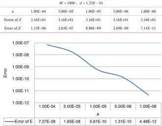
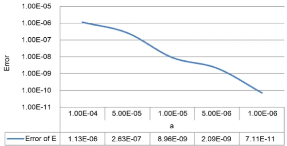
[image:8.595.207.538.448.704.2]

ka . When ka<1, the error of the solution is always less than 7.0E−08. Table 2 and Figure 2 show the results of solving the problem with M =1000 particles, when the distance between neighboring particles is d =1.25E−01 cm, and with different radius a. From Table 2, one can see that the error of the asymptotic solution is also very small when ka1, less than 1.13E−06, but greater than the previous case when M=125 for corresponding a. This time, the error is also decreasing rather quickly when the radius of the particles decreases from 1.0E−4 cm to 1.0E−6 cm. The small error when ka1 guarantees that the asymptotic formula (31) for the solution E is well applicable under this assumption.

Table 1. Error of the asymptotic solution E when M=125 and d=2.50E−01 cm.

125

M = , d=2.50E−01

a 1.00E−04 5.00E−05 1.00E−05 5.00E−06 1.00E−06 Norm of E 1.12E+01 1.12E+01 1.12E+01 1.12E+01 1.12E+01 Error of E 7.07E−08 1.65E−08 5.61E−10 1.31E−10 4.46E−12

Table 2. Error of the asymptotic solution E when M=1000 and d=1.25E−01 cm.

1000

M= , d=1.25E−01

a 1.00E−04 5.00E−05 1.00E−05 5.00E−06 1.00E−06 Norm of E 3.16E+01 3.16E+01 3.16E+01 3.16E+01 3.16E+01 Error of E 1.13E−06 2.63E−07 8.96E−09 2.09E−09 7.11E−11

[image:9.595.225.521.69.220.2]

DOI: 10.4236/ajcm.2017.74031 443 American Journal of Computational Mathematics

Figure 2. Error of the asymptotic solution E when M=1000 and d=1.25E−01 cm.

7. Conclusion

In this paper, we present a numerical method for solving EM wave scattering problem by many small impedance bodies. For illustration, numerical experiments are also provided. The solution to the EM wave scattering problem can be computed numerically and asymptotically using the described method, and the result is highly accurate if the assumption ka1 is satisfied.

References

[1] Ramm, A.G. (1992) Multidimensional Inverse Scattering Problems. Chapman & Hall/CRC, London, 51.

[2] Tsang, L., Kong, J.A. and Ding, K.H. (2000) Scattering of Electromagnetic Waves: Theories and Applications. John Wiley & Sons, Hoboken.

https://doi.org/10.1002/0471224286

[3] Ramm, A.G. (2005) Inverse Problems. Springer, New York.

[4] Stavroulakis, P. (2013) Biological Effects of Electromagnetic Fields: Mechanisms, Modeling, Biological Effects, Therapeutic Effects, International Standards, Exposure Criteria. Springer Science & Business Media, Berlin.

[5] Tran, N.T. (2013) Numerical Solution of Many-Body Wave Scattering Problem and Creating Materials with a Desired Refraction Coefficient. The International Journal of Structural Changes in Solids, 5, 27-38.

[6] Ramm, A.G. and Tran, N.T. (2015) A Fast Algorithm for Solving Scalar Wave Scat-tering Problem by Billions of Particles. Journal of Algorithms and Optimization, 3, 1-13.

[7] Ramm, A.G. (2010) Electromagnetic Wave Scattering by Many Small Bodies and Creating Materials with a Desired Refraction Coefficient. Progress in Electromag-netics Research M, 13, 203-215. https://doi.org/10.2528/PIERM10072307

[8] Ramm, A.G. (2013) Scattering of Acoustic and Electromagnetic Waves by Small Bodies of Arbitrary Shapes. Applications to Creating New Engineered Materials, Momentum Press, New York.

[9] Tran, N.T. (2017) Numerical Method for Solving Electromagnetic Wave Scattering by One and Many Small Perfectly Conducting Bodies. Kansas State University, Manhattan.