Union Resolution Performance of Frequency Modulation
Parameter Based on RWT for LFM Signals
Wenchen Li1, Huimin Yang1, Hong Li1, Mei Dan2, Xuesong Wang2, Shunping Xiao2
1National Major Laboratory of Complex Electromagnetic Environmental Effects for Electronic Information System, Luoyang, China; 2School of Electronic Science and Engineering, National University of Defense Technology, Changsha, China.
Email: [email protected]
Received July 22nd, 2012; revised August 24th, 2012; accepted September 7th, 2012
ABSTRACT
Union resolution performance of FM (frequency modulation) parameter based on Radon-Wigner transform (RWT) for multi-component LFM (linear frequency modulation) signals is studied. Firstly, the RWT output expression is offered, and the independent resolution performances of initial frequency and chirp rate are analyzed. Secondly, the RWT output approximate analytic expression is given based on quadratic Taylor’s series expansion, and the contour property is ana-lyzed. Contour can be used to picture the union resolution performance of FM parameter, and 2-D resolution perform-ance is studied based on approximate analytic expression, and the union resolution expression of FM parameter and resolution ellipse are offered. The simulation results validate the union resolution expression, and show that the union resolution can improve the resolution performance of multi-component LFM signals, contrasted with absolute resolu-tion performance. The paper can help the study of LFM parameter estimaresolu-tion and resoluresolu-tion performance.
Keywords: Multi-Component LFM Signals; Radon-Wigner Transform (RWT); Resolution Ellipse; Union Resolution of FM Parameter; Half-Power Lobe Width
1. Introduction
The LFM signal is widely applied in domains such as radar, correspondence and sound navigation. LFM sig-nal’s parameter estimation is an important research sub-ject in the electronic intelligence system, target motive parameter estimation and ISAR image. There are many literatures about LFM signal parameter estimation me- thod, such as estimation performance, the operating speed and the application, for example ML (Maximum Likelihood) method [1], polynomial phase transform (PPT) [2,3], Radon-Wigner transform (RWT) or the Wigner-Hough transform (WHT) [4-6], Radon-Ambi- guity transform (RAT) [7,8], Fractional Fourier trans-form (FrFT) [9]. RWT or WHT are the commonly used LFM signal parameter estimation methods. RWT method searches the straight line in the Wigner-Ville time-fre-quency distribution plane. The cross term can be sup-pressed effectively through the line integral in RWT, which is used to estimate the initial frequency and chirp rate of LFM signals, ulteriorly, the amplitude and phase information can be estimated.
The research of RWT resolution for LFM signal is the foundation for multi-component signal separation. And there are quite a few literatures about the RWT resolution. Simulation results in literature [8] show that the RAT
chirp rate resolution is 1.5T2 and 1.4T2 for the square-law and enveloping ambiguity respectively. Lit-erature [10] defines the nominal resolution with the main lobe of 3 dB width (half-power width), Literature [11] indicates the range-velocity union resolution with the ambiguity diagram’s 3/4 interception area. In summary, the resolution definition is disparate in different litera-tures, and the nominal resolution can reflect the resolu-tion performance on a certain extent, but not accurately.
ter union resolution and the resolution ellipse area are obtained. Finally, the simulation results indicate that the union resolution of FM parameter is higher than inde-pendent resolution.
2. RWT FM Parameter Estimation
2.1. LFM Signal ModelSingle LFM signal model is expressed by:
2
0 1 2
exp
x t A j a a t a t n t (1) where 0 t T ,A a a a, , ,0 1 2 are the signal scope, the phase, the initial angular frequency (or initial frequency) and the angle FM rate (or chirp rate) respectively. n t
is gauss white noise, whose mean is zero and variance is 2
.
2.2. RWT of LFM Signal
The essence of Radon transformation is to transform the straight line to the point in plane through the rotation axis projection integral, and a point coordinate corresponds the straight line slope and the slant range, then the detec-tion and estimadetec-tion are carried in this parameter spatial domain. RWT method transform the LFM signal from the time domain to the parameter spatial domain includ-ing the initial frequency and the FM rate.
The Wigner-Ville distribution [5] of x(t) is
, e
2 2
x
W t x t x t xp j d
(2)LFM signal chirp rate Ktan2a2, axis in-tercept 1, viz. initial frequency of .
According to the Wigner-Ville distribution character-istic of LFM signal, Radon straight line integral trans-formation is expressed by the straight line slope
h a t0
K and the axis intercept , the integral is done along the line h
Kt h
. Then the signal is transformed from time domain to the parameter spatial domain composed by initial frequency h and chirp rate K. The scheme of Ra-don transformation is shown in Figure 1. The RWT formula is expressed by:
, ,
exp d d
2 2
RW K h W t Kt h d dt
x t x t j Kt h t
(3)Using the integration variable replacement [12], the formula can be transformed into:
,
exp
0.5 2
d 2RW K h
x t j Kt ht t (4) Namely the two-dimensional integral of RWT model-ing can be transformed to the power spectrum estimation
O t
[image:2.595.312.539.342.577.2]h
Figure 1. Scheme of radon transform.
of the time domain dechirp signal [13]. And the best es-timation of K h, may be determined by the maximum value position of RW K h
,
1, 2 a a
, and obtain the estimation value a aˆ ˆ1, 2 of by the K h, parameter estima-tion.
3. RWT Resolution of Initial Frequency and
Chirp Rate
From formula (4), the RWT output of the noise-free LFM signal model x t
is expressed by:
2 2
RWT
,
RW K h A T F K h,
(5) where
2 1
2 RWT
2
sin , 2 0
, 2
, , 2
a h T
c a
F K h
F a
0
K K
(6)
2
exp exp
2
, F F
F
(7)
2exp 0
π
exp d
2
y
F y j x x
(8)2 1
2
2 1
2
2
2 π
2
2 π
a K a h
T
a K
a K a h
a K
(9)
where Fexp
y Fcos
y jFsin
y
, Fcos
y is Fresnel cosine integral and Fsin
y is Fresnel sine integral [12].
,
2 2RW K h A T
h
max when a1, K2a2. The half-power lobe width of the RWT output function, that is RWT
2 When ,
F K h
2 0.5
a K
1 2
0
, is shown in Figure 2.
3dB
x 2.0038
is obtained via interpolation methodfrom sinc x 41 2 in Figure 2(a). The half-power lobe width of h is:
3 3
2 4.0076
2 2
dB dB
x h
T T
(10)
Using Fexp
0 0, obtains:
2 2
2 2
2 2exp
, ,0
RW K h A T F A T F (11) where T 2a2K π.3dB 2.2290
is obtainedvia interpolation method from F ,0 21
K
2 in Figure 2(b). The half-power lobe width of is:
2 3
3 2
2π 7.8047
2
dB dB
K
T T
2 (12)
4. Taylor Formula and Character of the
RWT Function
4.1. Taylor Formula of the RWT Function
The RWT function’s main lobe reflects the RWT union resolution of initial frequency and chirp rate. In order to
(a)
[image:3.595.341.540.199.388.2](b)
Figure 2. Tangential plane of RWT function. (a)
4sinc x 1 2; (b) F
,0 21 2.obtain the main lobe analytic expression in the different high, the RWT function is indicated with the quadratic Taylor series expansion on the point with maximum value, which is h a 1 and K2a2. The Taylor ex-pansion of FRWT
K h,
is quite complex, so this articledirectly calculates the quadratic Taylor series of RWT output on the maximum value using the expression of
,
RW K h . The quadratic Taylor formula is expressed by [12]:
2 1
2 1
2 1
2 1
2 1
2 1
2
2 2
2 1
2
2
2 2
2
2
2
2 1
2
2
2 2
, ,
,
2
,
,
1 2
2
, 1
2
,
2
K a h a
K a h a
K a h a
K a h a
K a h a
K a h a
RW K h RW K h RW K h
K a
K RW K h
h a h
RW K h
K a
K RW K h
h a h
RW K h
1
K a h a
K h
(13)
From formula (4), when the noise-free input signal
model is
2
0 1 2
exp
x t A j a a t a t , 0 t T , the RWT function is:
2
0 0
, T T ,
RW K h A
F h K td d (14) where
2 2
1 2
,
1
exp 2
2 F h K
j a h t a K t
(15)
Via
21
2
, K a 1
h a
F h K
,
,
1
2 2
,
2
F h K
j t F h K
K
,
,
,
F h K
j t F h K
h
,
2
2 2
,
,
F K h
t F h
h
K
,
2
2 2 2 2
, 1
, 4
F K h
t F h
K
K ,
2
2 2
, 1
, 2
F K h
t t F h
K h
obtains these item in formula (13) as follows:
21
2 2 2
, K a
h a
RW K h A T
(16)
2 1 2 , 0 K a h aRW K h K
(17)
2 1 2 , 0 K a h aRW K h h
(18)
2 1
2 2 6
2 2 , 2 45 K a h a
RW K h A T
K
(19)
2 1
2 2 4
2 2 , 6 K a h a
RW K h A T
h
(20)
2 1
2 2 5
2
,
12
K a h a
RW K h A T
K h
(21) Taylor formula (13) is transformed into:
4 2 2 2 2 2 3 2 1 2, 1 2
45 2
12 12
T
RW K h A T K a
T h a T K a h a
1 (22)Obviously the RWT output is nonstandard quadratic surface, which can be proved to be nonstandard ellipse paraboloid.
4.2. The Contour Line Parameter Analysis of the Quadratic Taylor Formula
The RWT output is two-dimensional function of initial frequency and chirp rate, and the greatest value is A T2 2. The lobe characteristic of the RWT output function is reflected by the contour line along 2 2
contourA T
and the
cutting coefficient of contour line is 0contour 1. The output result is not the standard analytic expression, therefore the RWT cutting contour line is indicated by the quadratic Taylor formula, as follows:
21
contour 2
, , K a
h a
RW K h RW K h
(23)
Substitutes the quadratic Taylor formula, obtains:
2
2
2 2
1 2 2 1 2
a h a b K a c h a K a2 1 (24) where
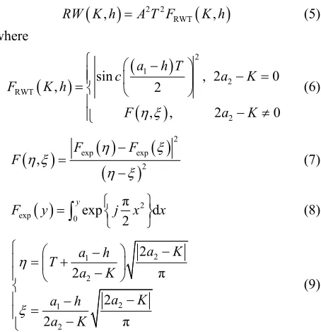
Using h a K 1, 2a2 as the center, and prescribing counterclockwise is positive, the coordinate system
1 2 2 h a h K a K
is counter-clockwise rotated with
angle , and the coordinate system x
y
is obtained,
shown in Figure 3.
1 2 cos sin 2 sin cos h a x K a y
(26)
1
2
cos sin
2 sin cos
h a x
K a y
(27)
In the coordinate system x
y
, Equation (24)
trans-forms into:
2 2
2 cos sin 2 sin cos
cos sin sin cos 1
a x y b x y
c x y x y
(28)when the item of xy is zero, the equation is standard ellipse, and obtains
2 2 2 tan 2 4 1 15 c T
a b T
(29)
And formula (28) is simplified to
2 2 2 2 2
2 2 2 2 2
cos sin sin 2
2
sin cos sin 2 1
2 c
a b x
c
a b y
(30)
It can be proved that the equation coefficient is more than zero, that is
2cos2 2sin2
sin 2 02 c
a b (31)
Therefore, the equation is the elliptic equation, the RWT quadratic surface is nonstandard ellipse paraboloid. 4.3. Contrastive Analysis of Quadratic Taylor
Formula and Actual Contour Line
In order to analyze conveniently, the performance of
[image:4.595.255.536.87.534.2]y x h K 1 a 2 2a K h
2 2 contour 4 2 contour 3 contour 12 1 45 1 12 1 T a T b T c (25)RWT resolution is characterized by half-power lobe width in this article. The half-power lobe contour line, which is obtained by quadratic Taylor formula, is the RWT output amplitude contour 2 2. By
2
2
K a 0, the half-power lobe width of h is:
3 contour
2 2 3.7495
12 1
dB
h
a T T
(32)
By h a 1 0, the half-power lobe width of K is:
3 2 contour 2
2 2 45 1 7.2609
dB
K
b T
T (33)
The result is close with the half-power lobe width 3dB 4.0076
h T
and 2
3dB 7.8047
K T
, which is
obtained directly by curve simulation and interpolation. There are two main error sources: The one is abbreviate of higher item, the other is cutting departure from the spot with maximum value. The half-power lobe width of the actual RWT output can be approached by adjustment the parameter contour, and the best revision interception coefficient contour is:
contour contour_h contour_K 2 0.6635
(34)
where contour_h,contour_K are obtained separately by the
half-power lobe width of h, K, the expression is ex-pressed as follows:
3 contour 3
2 12(1 )
dB h dB
h ρ h
T
_ (35)
3 2 contour_ 3
2 45(1 )
dB K dB
K K
T
(36)
Namely, when contour 0.6635, the lobe width using the quadratic Taylor formula is able to approach the ac-tual RWT output half-power lobe width, which is proved by the simulation result.
5. RWT Union Resolution of Initial
Frequency and Chirp Rate
The signal resolution is analyzed usually by two signals with equi-signal length, amplitude and initial time. The multi-component signal amplitude is A, the length is , namely are the constants, the signal position is , the i th component signal’s initial fre-quency is i and chirp rate respectively is
T a b c, , T
0 t
h K ii
1, 2
,its half-power cutting contour line is:
2
2
2 2 1
i i i
a h h b K K c h h K K i
(37) This formula can be reduced to:
2 2
2
2 1
i i
i i
e ah bK ah bK
f ah bK ah bK
(38)
where
2
2 1
1
2 2
1 1
2 2
c e
ab c f
ab
(39)
Defines
X e ah bK Y f ah bK
(40)
Obtains
1 2
1 2
X Y h
a e f X Y K
b e f
(41)
Therefore X Y, and both have corresponding relationships, formula (37) in coordinate system
, h K
,
X Y is circle equation.
2
21
i i i i
X e ah bK Y f ah bK
(42)
where, the circle point of the th component signal in coordinate system
i
,
X Y is e ah
ibKi
, f ah
ibKi
,and the circle track data can be generated by the circle equation, from which, we can get the corresponding contour line data h K, after the coordinate system conversion.
The two component signal’s FM parameters are 1 1, 2 2 respectively. According to the nominal resolution, two signals can not be distinguished if half-power contour lines have the intersection point in the coordinate system , otherwise two signals are distinguishable. In the coordinate system
,
h K h K,
,
h K
,
X Y , the contour line is circle. So long as the central distances of two circles are more than 2, the two LFM signals can be distinguished. The condition is described by:
2 2
2 1 2 1
2 2
2 1 2 1 4
e a h h b K K f a h h b K K
(43)
Inputting e f2, 2, the formula can be reduced to:
2 2
2 2
2 1 2 1
2 1 2 1 4
a h h b K K
c h h K K
(44)
Inputting , the resolution expression based on parameter is
2, ,2
a b c
2 4
2 2
2 1 2 1
3
2 1 2 1 contour
12 45
4 1 12
T h h T K K
T
h h K K ρ
where contour 0.6635
,
h K h K,
, and multi-component signal is able to be resolved, so long as the position of FM pa-rameter 1 1, 2 2 satisfies the above equation. Obviously in order to achieve the high resolution of initial frequency and chirp rate, the time length must be increased.
The union resolution of initial frequency and chirp rate may be indicated by the interception ellipse area.
contour
3 2 2 2π 1 24 15π
4 S
T
a b c
(46)
Obviously the resolution ellipse’s area is in reverse proportion with , related with the interception co- efficient
3
T contour
.
6. Simulation Results
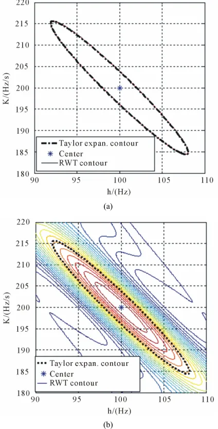
6.1. The RWT Output of Single Component LFM Signal
The signal model is:
exp
1 100 1002
x t j t t (47) The digital simulation result is given in Figure 4, where , , namely a = 0.5334, b = 0.2754,
c = 0.2845, and the FM parameter sampling interval is quite small in order to study the fine characteristic of RWT output. Figure 4(a) is the contrast of RWT half-power contour line and the Taylor’s expansion contour line in contour
0 t T
0. 1 T
6635
0.6635
. Figure 4(b) is the contour line view. It is indicated that the contour line two-dimensional superposition is very good for the two methods, therefore the RWT output half-power contour line is described well by the contour line equ
contour
ation in
. The results indicate simultaneously that the FM parameter estimation error is very small for a single component noise-free LFM signal.
6.2. The RWT of Multi Component LFM Signal The signal model is:
20 1 2
exp
x t A j a a t a t (48) The signal length is 1s, initial frequency independent resolution is , chirp rate independent resolution is 3 . The first component is:
4.0076
dB
h
3dB 7.8047
K
21 exp 1 100 100
x t j t t (49) The second component is:
22
1
exp 2 100 d 100 d
2
x t j h t K t
(50)
The RWT resolution performance of two component LFM signals is studied by changing the initial frequency and chirp rate of the second component separately in
(a)
[image:6.595.318.530.88.505.2](b)
Figure 4. Contrast of Taylor formula and actual contour line of single component LFM signal. (a) Is the contrast of RWT half-power contour line and the Taylor’s expansion contour line in ; (b) Is the contour line view.
contour0.6635
what follows.
6.2.1. Independent Resolution of Initial Frequency and Chirp Rate
The simulation results of initial frequency and chirp rate independent resolution are shown in Figure 5, including contour map and projection view. Two LFM signals with same chirp rate and different initial frequency (dh h3dB, dK 0) are shown in Figure 5(a). Two
(a)
[image:7.595.326.520.78.684.2](b)
Figure 5. Contrast of Taylor formula and actual contour line of multi component LFM signal. The second component in formula (50) is (a) dh = ∆h3dB, dK = 0; (b)dh = 0, dK = ∆K3dB.
coupling of the very near two LFM signals cause the RWT output peak position to be away from the primary position, which incurs FM parameter estimation devia-tion. Simultaneously the further simulation results indi-cate that the different phase item 0 in the two LFM signals causes the different peak position errors, and the starting phase items of the two LFM signals affect the pa-rameter estimation errors, but the LFM signals are distin-guishable if the distinguishing condition is satisfied. Therefore the nominal resolution reflects the resolution performance to a certain extent. For single component LFM signal or multi-component LFM signal with the great FM parameter space interval in RWT, the RWT
a
(a)
(b)
(c)
Figure 6. Union resolution of initial frequency and chirp rate of multi component LFM signal. The second compo-nent in formula (50) is (a) dh = ∆h3dB/2, dK = 0; (b) dh = 0,
[image:7.595.65.278.84.513.2]parameter estimation error is related with SNR input. On the other hand, for the distinguishable multi-component LFM signal with the close FM parameter space interval, FM parameter estimation error is related with both SNR and other component signal’s parameter.
6.2.2. Union Resolution of Initial Frequency and Chirp Rate
Union resolution of multi-component LFM signal is studied and simulation results are shown in Figure 6, including contour map and projection view. (a) The sec-ond component dh h3dB 2, , and the signals
cannot be distinguished by RWT method; (b) The second component ,
dK 0
dh0 dK K3dB 2 , and the signals
cannot be distinguished by RWT method; (c) The second components with the initial frequency and chirp rate are all half of independent resolution, namely dh h3dB 2
and dK K3dB 2. It is obviously the two LFM signals
are distinguishable by RWT method. The simulation re-sults confirm the superiority of the FM parameter union resolution.
As to two multi-component signals with close FM pa-rameter space, the estimation error is big when the am-plitudes are similar, and the optimum parameter esti- mation of various components can be obtained by Relax iteration method [14]. On the other hand, if the intensity difference of two signals is distinct, the strong signal suppresses the weak signal, therefore the CLEAN tech-nology must be used to extract the signals [15].
7. Conclusion
Union resolution performance of FM parameter based on RWT for multi-component LFM signals is studied in this paper. Firstly, the RWT output expression is given, and the independent resolutions of initial frequency and chirp rate are analyzed. Secondly, the RWT output approxi-mate analytic expression is given by Taylor series expan-sion. The contour line property is analyzed and the con-tour line is deviation, which caused by approximation in Taylor expansion, is revised. Contour can be used to picture the union resolution performance of FM parame-ter of RWT, and 2-D resolution performance is studied based on approximate analytic expression. The union resolution expression of FM parameter and resolution ellipse area is offered. Finally the simulation results in-dicate that the union resolution of FM parameter is higher than independent resolution. The research in this paper can help the study of LFM parameter estimation and resolution performance.
REFERENCES
[1] T. J. Abatzoglou, “Fast Maximum Likelihood Joint Esti-mation of Frequency and Frequency Rate,” IEEE
Trans-actions on Aerospace and Electronic Systems, Vol. 22, No. 6, 1986, pp. 708-715.
[2] S. Peleg and B. Porat, “Linear FM Signal Parameter Es-timation from Discrete-Time Observations,” IEEE Trans- actions on Aerospace and Electronic Systems, Vol. 27, No. 4, 1991, pp. 607-615. doi:10.1109/7.85033
[3] S. Peleg and B. Porat, “Estimation and Classification of Polynomial Phase Signals,” IEEE Transactions on Infor- mation Theory, Vol. 37, No. 2, 1991, pp. 423-430. doi:10.1109/18.75269
[4] J. C. Wood and D. T. Barry, “Radon Transformation of Time-Frequency Distributions for Analysis of Multi-Com- ponent Signals,” IEEE Transactions on Signal Processing, Vol. 42, No. 11, 1994, pp. 3166-3177.
doi:10.1109/78.330375
[5] J. C. Wood and D. T. Barry, “Linear Signal Synthesis Using the Radon-Wigner Transform,” IEEE Transactions on Signal Processing, Vol. 42, No. 8, 1994, pp. 2105- 2111. doi:10.1109/78.301845
[6] S. Barbarossa, “Analysis of Multi-Component LFM Sig-nals by a Combined Wigner-Hough Transform,” IEEE Transactions on Signal Processing, Vol. 43, No. 6, 1995, pp. 1511-1515. doi:10.1109/78.388866
[7] M. S. Wang, A. K. Chan and C. K. Chui, “Linear Fre-quency-Modulated Signal Detection Using Radon-Am- biguity Transform,” IEEE Transactions on Signal Proc-essing, Vol. 46, No. 3, 1998, pp. 571-586.
doi:10.1109/78.661326
[8] W. C. Li, M. Dan, X. S. Wang, D. Li and G. Y. Wang, “Fast Estimation Method and Performance Analysis of Frequency Modulation Rate via RAT,” International Con- ference on Information and Automation, Changsha, China, 20-23 June 2008, pp. 144-147.
doi:10.1109/ICINFA.2008.4607984
[9] L. B. Almeida, “The Fractional Fourier Transforms and Time-Frequency Representations,” IEEE Transactions on Signal Processing, Vol. 42, No. 11, 1994, pp. 3084-3091. doi:10.1109/78.330368
[10] M. I. Skolnik, “Radar Handbook,” 2nd Edition, McGraw- Hill Publishing Company, New York, 1990.
[11] A. W. Rihaczek, “Principles of High-Resolution Radar,” McGraw-Hill Publishing Company, New York, 1969. [12] L. X. Wang, D. Z. Fang, M. Y. Zhang, et al.,
“Mathemat-ics Handbook,” Higher Education Publishing Company, Beijing, 2004.
[13] W. P. Li, “Wigner Distribution Method Equivalent to Dechirp Method for Detecting a Chirp Signal,” IEEE Transactions on Acoustics, Speech, Signal Processing, Vol. 35, No. 8, 1987, pp. 1210-1211.
[14] Y. M. Zheng and Z. Bao, “Autofocusing of SAR Images Based on Relax,” IEEE International Radar Conference, Alexandria, 7-12 May 2000, pp. 533-538.
doi:10.1109/RADAR.2000.851890
[15] J. Tsao and B. D. Steinberg, “Reduction of Side Lobe and Speckle Artifacts in Microwave Imaging: The CLEAN Technique,” IEEE Transactions on Antennas and Propa- gation, Vol. 36, No. 4, 1988, pp. 543-556.