Methodology and analysis for the recognition of tumour tissue based on FDG PET

Methodology and analysis for the recognition of

tumour tissue based on FDG-PET

Master Thesis

in Applied Mathematics

by

G.R. Lagerweij

April 18, 2012

Chairman: Prof. Dr. H.J. Zwart Prof. Dr. A.A. Stoorvogel

Abstract

For diagnosing the cause of a patient’s illness medical images are used more and more. Each medical problem can be visualized with its own specific image. For the detection of tumour tissue the main medical image is a Positron Emission Tomography (PET) image.

A patient with suspicious tissue is injected with a radio-active substance. This active substance will decline and a positron is formed. This element will bump into an electron and two gamma photons appear due to this collision. When two opposite detectors in the scanner detect an arrival of a gamma photon within a certain time interval, the computer receives a signal. The intensity of these signals gives an indication of the density and location of the radio-active substance.

Active organs and tumour tissue attract this radioactive substance since it is combined with glucose, therefore these parts are visible on a PET scan. So by making a PET scan the location and amount of the tumour tissue can be determined.

Not all photons are detected correctly, so noise arises. This noise affects the accuracy of the image. It is important to get an indication of the effect and consequences of the noise.

Besides the noise an extra difficulty of a PET image is the difference between two various PET images, each patient has its own PET image with specific intensity values. The reason is that each patient is different by gender, age or level of metabolism. Another difficulty is the origin of a high intensity pixel, a pixel can have a high intensity for many reasons. For example, a high intensity pixel describes a part of an active organ, but it can also be caused by an infection. Therefore it is very difficult to determine whether or not a pixel is suspicious based on its intensity only.

A literature study on PET images and the effect of noise is performed. A PET image looks like a photo, so perhaps it is possible to use algorithms used in the photo-industry, unfortunately this does not seem possible. There are big differences between pictures and PET images, the main difference is the number of pixels. One slice of a PET image exists of 168×168 pixels, this slice is a vertical

cross-cut of your body. Note that a PET scan is three-dimensional, therefore it consists of multiple two-dimensional slices.

A normal photo has at least twice as much pixels as a PET image, therefore a PET image is not accurate enough and that is why it is so important to distinguish tumour tissue from the noise. To illustrate this, one strange pixel can be a tumour of 0.5cm2.

In a photo it is easy to detect a strange pixel, because of the precision. This strange pixel can be determined based on its neighbors, a white pixel stands out from a group of black pixels. In a PET image it is unknown whether a pixel should be white or black.

Other algorithms for clustering pixels into groups based on their gradation are not useful but still it is important to understand the effects of the noise. Therefore the distribution of the noise is investigated and the data from a PET scan is estimated with a distribution. This results in a difficult distribution which can not be implemented properly, therefore instead a normal distribution is used to perform the simulations.

The methodology of the simulations and the performed steps are described extensively. From the data set of a phantom study a normal distribution is estimated. With this distribution a data set with correlated random values is generated. All pixels with a high intensity, the outliers, are determined for a certain percentage (1% or 5%) and one pixel is increased to a certain value.

An outlier has more correlation with its neighbors and hence the difference in intensity between such a pixel and its neighbors is relatively small. For an increased pixel it is the opposite; the difference in intensity will be relatively large. The simulations support this hypothesis. These differences in inten-sities are used to determine confidence intervals for both outliers and increased pixels. The next step is to find a (variable) criterion based on these confidence intervals. The best criterion is based on a trade-off between well judged pixels and wrongly judged outliers. Wrongly judged outliers are actual outliers which are identified as suspicious pixels.

The simulations work rather well, still the question is whether it is a realistic implementation of PET images. To investigate this, a validation of the distribution for the noise is performed. The theoretical values for the increased pixel can be derived using a normal distribution. The experimental values converge within 1000 simulations to these theoretical values, this is true for both the expected value and the variance of the distribution of an increased pixel.

The derivation of the theoretical values for the outliers is a lot harder, the distribution of an outlier changes since the data set has changed (only the outliers are evaluated, not all pixels). We have to deal with a conditional probability because of the condition that the intensity of the pixels is above some value. It turns out that the experimental values of the outliers converge a lot slower to their theoretical values (within 2000 simulations), but also these values converge.

The results of the simulation are promising, however an optimal criterion can not be established because it is highly dependent on the situation and preferences of the doctor. On the other hand the derived percentages for correctly and wrongly judged pixels are also promising.

Next the methodology used in the simulations is applied on PET images. These results are less conve-nient because the necessary confidence intervals can not be established. Therefore the results of applying the methodology on PET images give rise for further research.

Preface

Nothing about my life has been easy, but nothing is gonna keep me down, cause I know a lot more today, than I knew yesterday,

so I am ready to carry on.

It is over, I am finishing my study and I will have to say goodbye to Enschede. It is amazing how fast the years past by.

More than six years ago I moved to Enschede, a big change in my life. Still I remember the intro-duction, dancing on a table though that was never the plan, for the first time in my life I went to the disco, got nights with less sleep then ever but it was wonderful. I have been a member of the board of study association W.S.G. Abacus. It was an incredible year, I learned a lot, earned some study credits, had long evenings (and nights) and laughed a lot with everybody. After this year, I went on studying and now almost three years later, I am finishing my final project.

In this way my autobiography looks nice, but that is not totally true. I had to work very hard to get to this point. The costs were a lot of tears, sweat, frustrations, blood and conversations with people. Sometimes I though I had some syrup to attract difficult situations. All these “bad” things have resulted in something nice; I grew up. They have made me stronger, more secure and positive. The uncertain and litte girl has changed into a powerful woman.

After almost six years of working I am glad that it is over. I am grateful for all the things I have learned, all the people I have met and all the things I have experienced.

Contents

Abstract 3

Preface 5

List of Tables 9

List of Figures 11

List of Symbols 13

1 Introduction 15

1.1 Positron Emission Tomography . . . 15

1.2 FDG-PET . . . 16

1.3 Reconstruction . . . 16

2 Problem formulation 17 2.1 Noise on PET images . . . 17

2.2 Goal . . . 17

3 Literature review 19 4 Derivation of the noise model 21 4.1 Distribution . . . 21

4.2 Correlation . . . 26

4.3 Covariance matrix . . . 28

4.4 Random values from the distribution . . . 31

5 Simulations 33 5.1 Determining an outlier . . . 33

5.2 Distance . . . 33

5.3 One increased pixel . . . 34

6 Validation of the model 39 6.1 Theoretical values of an increased pixel . . . 39

6.2 Theoretical values of an outlier . . . 41

6.3 Conditional variance . . . 42

6.4 Validation of the values . . . 43

7 Results 45 7.1 Judgement of the outliers . . . 45

7.2 Variation in the simulations . . . 47

7.3 PET images . . . 49

8 Conclusion 53 8.1 Simulations . . . 53

8.2 PET images . . . 53

9 Discussion and further research 55

Acknowledgements 59

Appendices 61

A Definitions 61

B The increased pixel 63

B.1 Expectation . . . 63

B.2 Variance . . . 63

C Tables 67 C.1 Validation values for expected value . . . 67

C.2 Constant criterion . . . 67

C.3 Confidence interval for three models . . . 67

C.4 Different variable criterion . . . 67

C.5 Three different models . . . 68

C.5.1 vpixel= 1.25·vlimit . . . 68

C.5.2 vpixel= 1.5·vlimit . . . 68

D Covariance matrix 71

List of Tables

1 Correlation for eight neighbors . . . 28

2 Correlation for ten neighbors . . . 29

3 First round of neighbors . . . 29

4 Second round of neighbors . . . 29

5 Different intensity values for two rounds of neighbors and different percentage outliers . 35 6 Four direct neighbors and their location . . . 35

7 Difference in distance for two percentage outliers . . . 36

8 95% Confidence interval for two percentage outliers . . . 36

9 Experimental and theoretical expected values for 5% outliers performed by 2000 simulations 43 10 Discrepancy of the standard deviation for 5% outliers andvpixel= 1.5·vlimit . . . 44

11 Constant criterion, withvpixel= 1.5·vlimit . . . 46

12 Variable criterion, withvpixel= 1.5·vlimit . . . 47

13 Confidence interval for 5% outliers and three models . . . 48

14 Three models with a constant criterion for two percentage outliers . . . 48

15 Three models for 5% outliers with a two variable criterions . . . 49

16 Correlation coefficient for two (most likely) healthy livers . . . 50

17 Absolute value of the relative discrepancy between correlation coefficients for two (most likely) healthy livers . . . 51

18 Correlation with horizontal neighbors . . . 51

19 Correlation with vertical neighbors . . . 51

20 Correlation coefficients for a sick patient with a (most likely) healthy liver . . . 51

21 Correlation coefficients fornhorizontal and vertical neighbors . . . 52

22 Absolute value of the relative discrepancy of the expected value for 5% outliers and vpixel= 1.5·vlimit . . . 67

23 Constant criterion with values forvpixel . . . 67

24 Confidence interval for 1% outliers for the three models . . . 67

25 Variable value as criterion, withvpixel= 1.25·vlimit . . . 68

26 Three models for 5% outliers with a variable criterion andvpixel= 1.25·vlimit . . . 68

27 Three models for 1% outliers with a variable criterion and withvpixel= 1.25·vlimit . . . 68

28 Three models for 1% outliers with a variable criterion and withvpixel= 1.5·vlimit . . . 68

List of Figures

1 Coincidence events of a PET image [21] . . . 15

2 Histogram of the phantom data including the noise . . . 22

3 Histogram fit of the noise . . . 23

4 Plot of normal probability . . . 23

5 A plot of a (skew) normal distribution [9] . . . 24

6 A plot of four hermite polynomials [7] . . . 25

7 A plot of two determined Hermite polynomials and the data . . . 26

8 A plot of two determined Hermite polynomials . . . 27

9 Plot of the matrix of the phantom study . . . 28

10 Uncorrelated noise . . . 32

11 Correlated noise . . . 32

12 Empirical rule of normal distribution [5] . . . 33

13 Histogram of the squared distance for 10% outliers . . . 39

14 2D plot for the joint probability function . . . 43

15 Histogram for a limit of 1% . . . 45

16 Histogram for a limit of 5% . . . 45

17 PET image of a liver from a patient . . . 49

18 Young patient . . . 50

19 Old patient . . . 50

List of Symbols

Symbol Description Page

¯

x Mean value 21

s Sample standard deviation 22

s2 _{Sample variance, can be determined by squaring the (sample) standard deviation s 30}

ρx,z Correlation coefficient between the pointsx and z 27

pspace Length between two pixels, approximately 4.07283 mm 28

vlimit Limit value for a certain percentage outliers 33

d Difference between the intensity of a point and its neighbor 35

d2 Squared distance between a point and its neighbor 35

¯

d Sum of all distances, for all neighbors, divided by the number of neighbors 34 dr1 Sum of all distances for round 1 neighbors, divided by the number of neighbors 34 dr2 Sum of all distances for round 2 neighbors, divided by the number of neighbors 34

do Average distance for an outlier 34

dp Average distance for an increased pixel 34

pgood Percentage well judged suspicious pixel 45

pwrong Percentage wrongly judged suspicious pixel 45

vpixel The intensity of the increased pixel 46

CIOL The left limit value for the confidence interval for an outlier 45

CIOR The right limit for the confidence interval for an outlier 46

CIPL The left limit for the confidence interval for an increased pixel 45

CIPR The right limit for the confidence interval for an increased pixel 45

kin The difference between the right limit of the confidence interval for an outlier (CIOR) 46

1

Introduction

The subject of this thesis is a specific type of medical images, this chapter presents the background of these images.

1.1 Positron Emission Tomography

We begin with a short introduction on PET images in general. The abbreviation PET stands for Positron Emission Tomography, a technique that visualizes the distribution of a radioactive substance in a human body, more precisely this substance consists of a positron emitter. A radioactive substance is characterized by its decay after some time, during the decline of the active substance used in PET studies, a positron is formed. This positron moves and collides with an already present electron. Both particles disappear (annihilation) and two gamma photons arise, these gamma photons move freely but in opposite directions.

The patient is positioned in a ring with gamma detectors. As soon as two opposite located detectors detect a trigger (an arrival of a gamma photon) within a certain time interval, a signal is send to the computer. This way, it is possible to determine the location and amount of annihilation.

The detection of two triggers at exactly the same time instant is called a coincidence event [2, 21]. Coincidence events in PET can be divided into four categories: true, scattered, random and multiple. All four coincidences are shown in Figure 1.

Figure 1: Coincidence events of a PET image [21]

coincidence event. This coincidence time-window is in the order of nanoseconds.

For a true event photons do not have any interaction with other photons before detection. Furthermore no other events are detected within the specific coincidence time-window.

For a scattered coincidence, see Figure 1 right top, one of the photons has a changed direction during the process. This type of a coincidence adds noise to the actual signal and results in an incorrect posi-tioning of the event.

The third form of coincidences is called random events. These events occur when two photons, not com-ing from the same annihilation event, are detected within the coincidence time-window of the system. These random coincidences also add noise to the data.

Multiple coincidence events are the last form of coincidence events. These events include that three or more photons are detected simultaneously within the same coincidence time-interval. Again this type of coincidences causes noise on the data.

1.2 FDG-PET

PET images have their main application in determining the presence of tumour tissue and its severity rate. The amount and type of nuclear substance used differs per patient and tissue. For investigat-ing suspicious tissue a radioactive substance combined with an amount of fluorine-atoms is used, this substance (2-fluoro-2-deoxy-D-glucose) is abbreviated with FDG. Human body parts that consume a lot of energy absorb this substance. Examples of organs that consume a lot of energy are the brains, the heart and the liver. Not only active organs will transmit radiation but the tumour tissue will too. This is because tumours are active and fast growing tissues and will therefore attract more glucose than the healty tissues. It is also likely to find FDG in the bladder and kidneys because the radioactive substances will be secreted in these organs.

Due to PET scans it is possible to visualize the location of the radioactive substance FDG and with this to detect the location of possible suspicious tissue.

1.3 Reconstruction

As described in Subsection 1.1 the number of coincidence events gives an indication of the location of the annihilation, only a limited number of the released gamma photons reach the detectors. The remaining photons stay in the human body. Of all the photon couples that reach the ring of detectors only a small part can be used to locate the annihilation (the true coincidence events). It is not true that all photons go in a straight direction, because sometimes a photon arrives with a graduated corner (scatter). Therefore the precise location of this annihilation is difficult to establish.

After the PET scanner has detected all coincidences a reconstruction method is applied [12], after this reconstruction the PET image is ready. Now the distribution of the injected radioactive fluid in the patient’s body is known.

The limited number of photons causes another uncertainty and therefore additional noise arises. Since it is not possible to detect all released photons, the effect of noise is large. One possible way of improving a PET image is upgrading the reconstruction method, but the way of reconstruction differs per scanner. So this would not lead to a general solution which we desire.

2

Problem formulation

Although it is not always obvious, every signal (e.g. electrical) is affected by noise. The effect of noise can be very small, but it can also be large. Roughly speaking, noise is nothing more than a perturbation of the desired signal, an example of noise on a signal is “snow” on a television. High noise levels can change the meaning of a message in (electronic) communication, which may result in making wrong decisions. Therefore it is important to know the amount of noise on a signal.

2.1 Noise on PET images

Unfortunately the effect of noise is large in medical imaging, so it is hard to distinguish the actual signal from the noise. Particularly the noise in FDG-PET images plays an important part. An FDG-PET image is used to detect suspicious tissue like a tumour, this detection depends on the contrast between the activity of the tumour and its background. The tumour detection becomes easier if the noise level is low. However, the noise is affected by many factors; gender, age, metabolism level, injected dose radioactivity, etc.

As described in Chapter 1, it is difficult to determine the exact location of the annihilation. A second difficulty is the unknown amount of annihilations, hence there are already uncertainties before the re-construction takes place. Thus the rere-construction method will affect the data with noise.

The precise reconstruction method is unknown because of the confidentiality of the manufacturer, therefore it is not that easy to upgrade the reconstruction method. Some researchers have attempted to reproduce the reconstruction method. However for reducing the effect of noise in PET images the details from the following (literature) studies are not sufficient: [19, 24, 26].

The question remains how to distinguish the noise from the actual signal. A disadvantage of PET images is that a large pixel intensity does not mean that this pixel is a tumour, for example a pixel in the liver-area or brain-area can also have a high intensity. A high intensity pixel can even be an infection. For this reason, it turns out that it is rather impossible to create a probability distribution of tumour and of not-tumour tissue. The question there is whether it is possible to say with a certain probability that a pixel is noise or not.

2.2 Goal

3

Literature review

Before it is possible to acquire more information from the FDG-PET images, it is necessary to perform some research on the available literature. In this chapter we give an overview of this research and the results on improving FDG-PET images. After this literature study the methodology we worked with is explained in Chapter 4.

It is a known fact that FDG-PET images have a low resolution. From early literature studies it is known that the effect of noise on PET images is large. Therefore the aim is to find a method that will reduce the effect of noise ion FDG-PET images.

The literature study has to be taken widely. There is not much literature of PET images in combination with noise and improving the quality of the images. A question that comes up naturally is, what the difference between a picture of a photo camera and a PET image is. Can an algorithm of a photo camera be used for improving a PET image?

The main difference between a photo and a PET image is the resolution. A photo has a larger resolution, which means more pixels in one image. The format of one pixel of a photo is smaller and therefore a picture of a photo is more precise. Another difference is the prior knowledge of the photo. If you see a photo with a white pixel surrounded by black pixels, you know it is not correct. The reason that you visualize this problem, is the comparison with the neighbors of this deviant pixel. In a PET image this is not possible because based on its neighbors only, a deviant pixel is not necessarily good, i.e. healthy. It is likely that the neighborhood has some influence, but taking the neighborhood as real is not right. The neighborhood can as well be effected by noise. Therefore it is difficult to apply algorithms or methods that are used in the photo-industry.

A second point of interest is the correlation between the input and noise. It is known that the activity concentration is related to the signal to noise ratio (SNR) and the noise equivalent counts (NEC) [15]. This should be observed by determining the right algorithm. The situation is easier when the noise of a picture is not statistically dependent on the original image. In that case it is possible to recover the actual image from a noisy image [22], but earlier research shows that the noise and the original image are dependent.

A further literature study shows another way for detecting and clustering (deviant) points [13, 16, 17]. For example, the algorithm Fuzzy C-Means (FCM) [14] clusters all points into groups with a certain degree. The number of groups is defined by the user. The neighborhood for each investigated pixel is taken into account.

The objective function for partitioning a set {xk}Nk=1 intocclusters is given by [11, 18, 28]:

J = c ! i=1 N ! k=1

up_ik||xk−vi||2 (1)

with {vi}ci=1 the prototypes of the clusters, p as weighting exponent on each fuzzy membership and {uik}Nk=1 =U the partition matrix. This partition matrix is of the form

U =

"

uik ∈[0,1]

# # # # # c ! i=1

uik = 1 ∀k and 0< N

!

k=1

uik < N ∀i

$

. (2)

changes. The change can be an addition in the form of a feature direction for the pixel intensity or a distance attraction for the spatial position of the neighbors which depends on the structure of the neigh-borhood. Both additions affect the attraction between the neighborhood and the investigated pixels. Taking a kernel operator instead of the absolute value of the difference [28] can also be a modification. One of the Fuzzy C-Mean [11] methods is programmed in Matlab by a former student of the University of Twente. The BCFCM (Bias Corrected Fuzzy C-Means) algorithm is tested on MRI data and the results are good. The code is likewise applied on PET data, but the results are not hopeful. After some research and a meeting with a professor of Electrical Engineering (Prof. Dr. F. van der Heijden), it is clear that there is just one possibility of using an FCM method. The PET data must satisfy the constraint that the two (or more) probability distributions have a small relatively overlap. If the overlap is large, it is hard to distinguish pixels from each other.

In our case, clustering deviant pixels from normal pixels, the goal is to find a criterion for whether a point is suspicious or not. In most cases a suspicious pixel is tumour tissue. Therefore we have to deal with the probability distributions of normal tissue and tumour tissue. A pixel with a high intensity is not automatically suspicious. For example, pixels with high intensity in the brains have another interpretation than high intensity pixels in the liver. A pixel with a high intensity in the brain can be a tumour, but in the liver it is not. The reason could be for example the difference in metabolism. The intensity gives an impression of the metabolism level in tissue. Brain tissue has a higher level of metabolism than liver tissue.

We can conclude that it is very difficult to realize a probability distribution function of tumour tissue and one of not-tumour tissue that do not overlap.

To summarize, it is not possible to use a FCM method for clustering PET data into groups, because of the overlap in their probability density distributions. Another reason for not using a clustering method is the problem with the neighbors. As stated before it is not correct to eliminate a deviant pixel because of its neighborhood.

So, it seems that changing our approach is required. It is not likely that the solution for the de-tection of deviant pixels on PET image can be found in the available literatue.

4

Derivation of the noise model

Since some parts of the body absorb more nuclear substance than others, the resulting PET image is heterogeneous. This means that the image exists of roughness, which are causes by the presence of organs, the level of metabolism and the type of patient. As described in Chapter 3 not much literature is known on PET images in combination with noise. It is difficult to determine the effect of noise because of the rugged character of the PET images.

First we will focus on homogeneous images which have a constant input. A homogeneous PET image can be made by filling a phantom with a radioactive fluid and scanning this phantom. A phantom is a body without contents, e.g. a sphere, a bottle or a bucket. In our case this is a cylinder filled with water and the radioactive substance FDG. These scans are normally used for the reliability of the PET camera.

Literature shows that a homogeneous PET image has approximately a Poisson or Gaussian distribution [25, 27]. Does this estimated distribution describes the noise correctly? Can this estimated distribution be used for detecting deviant pixels? These question will be answered in the next subsection.

In the next subsection a distribution of the noise is estimated. A question which we want to answer is; does it agree with the results found in [25, 27]?

4.1 Distribution

Based on the phantom-studies it is possible to determine the distribution of the noise. In the ideal sit-uation the determined signal of the PET scan equals the injected radioactive substance. The difference between these two signals is the noise.

If the distribution of the noise is known, it is possible to neglect (a large part of) the effect of the noise on the signal. This cause the actual signal to become visual and therefore the determination of suspicious pixels is possible.

There are several phantom-studies available for determining the distribution of the noise. These studies also include different input activities, which helps to determine the precise effect of the activity on the distribution.

x := 1

N

N

!

i=1

xi (3)

Unfortunately, these studies show some curious phenomena. For instance, the difference between the mean, see (3), of the picture and the injected activity is large. For reliability reasons, the difference between these two numbers must be smaller than 10% of the input value. One reason for this difference might be caused by the rescale slope. This slope transforms the pixel values of the image into values which are meaningful for the application. This is required for the image to present the right intensity values measured in the human body.

After some more studies, we have decided to take only a recent phantom study and not to use the other studies. The difference between the mean of this study and its input value is less than 5%, which is acceptable. There is only one negative consequence of using only this (new) data set; now it is not possible to take a look at the effect of different radio activities as input.

A normal PET study of a patient has a data matrix of 168×168×374. The actual data set of

matrix of 25×25×55 pixels is taken because the borders of the PET scan are not suitable. Therefore

the innermost part of the PET scan with a size of 25×25 pixels is taken. For all calculations, only one

slice is chosen which results in a data matrix of 625 pixels.

First a histogram is plotted for this particular slice. This histogram gives an indication of the probabil-ity densprobabil-ity function. Based on the histogram our hypothesis is that the data set is distributed normally with a certain mean and standard deviation. The mean of the noise will be zero, because the average intensity of the image has to be approximately the input, i.e. the injected radio-activity. And since the input is constant, the average of the noise becomes zero. The common estimation for the standard deviation is given by (4)

s :=

% & & ' 1

N₋1

N

!

i=1

(x₋xi)2, (4)

with ¯x the mean value. We remark that the standard deviation is different for each study, therefore for

each patient. Further details about the difference for the standard deviation are explained later.

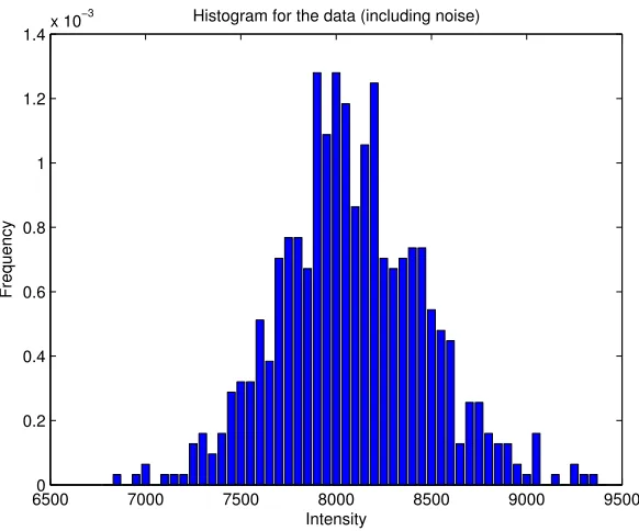
65000 7000 7500 8000 8500 9000 9500

0.2 0.4 0.6 0.8 1 1.2 1.4x 10

−3 _{Histogram for the data (including noise)}

Intensity

Frequency

Figure 2: Histogram of the phantom data including the noise

The histogram alone, see Figure 2, is not sufficient to determine the distribution. There are several tests for fitting a distribution to a dataset, see Matlab [1] for some demos.

The null-hypothesis is that the noise is distributed normally. The alternative hypothesis H1 is that

the distribution is arbitrary. The used tests, Kolmogorov-Smirov and Chi-Squared, reject the null-hypothesis several times. The corresponding p-values arepKS = 0 andpχ2 = 4.3926·10−20.

The only conclusion that can be taken is that the noise is not distributed normally.

−15000 −1000 −500 0 500 1000 1500 100

200 300 400 500 600 700 800

Noise data

Intensity

Frequency

Figure 3: Histogram fit of the noise

Figure 3. Still these outliers need to be judged whether they are innocent or suspicious.

In Figure 3 the histogram of the noise together with an estimated normal density function is drawn. This is one of the many applications of Matlab for fitting a distribution through data. Another appli-cation creates a normal probability plot of the data. For our noise data this plot is shown in Figure 4. This figure shows that the outliers are not fitted by a normal distribution.

Figure 4: Plot of normal probability

The box plot shows that de data is not distributed normally, since for a normal distribution it is allowed that 0.7% of the data is outlier whereas the PET data has 1.6% outliers.

The skewness and kurtosis of the distribution are also calculated. These numbers are a measure of skewness of the distribution and their formulas can be found in Equation (5) and (6).

skew :=

(N

i=1(xi−x)3

(N −1)s3 (5)

kurtosis :=

(N

i=1(xi−x)4

(N −1)s4 −3 (6)

The skewness says something about the number of outliers. It is not odd that the noise shows skewness because of the large number of large outliers. The skewness is that large that the noise can not be distributed normally and hence the noise could have a skew normal distribution, see Figure 5. Investi-gating this possibility will cost a lot of time because of the complexity of determining its parameters. Secondly there is not much known about a skew normal distribution, it is hard to say some about the distribution and its behavior. Therefore the skew normal distribution is not chosen as the distribution for the noise.

Figure 5: A plot of a (skew) normal distribution [9]

All together we can conclude that the data is not distributed normally.

Although the data is not distributed normally, it has strong similarities with a normal distribution, see Figure 3. In probability theory and combinatorics special polynomials are known, these polynomials are named after Charles Hermite [8].

The probabilists’ Hermite polynomials are of the following form:

Hn(x) = (−1)ne

x2

2 d

n

dxne

−x2

2 . (7)

polynomials. Figures 3 and 4 show that the number of outliers is the main reason why a normal dis-tribution does not fit. To get a feeling for these polynomials, in Figure 6, the Hermite polynomials of degree zero, one, two and three are plotted.

Figure 6: A plot of four hermite polynomials [7]

The aimed Hermite polynomial must be a probability density function, which means that the area under the function must equal one. Calculating the area under a probability density function means taking the integral from −∞ to∞, i.e.)_−∞∞ f(x)dx=_&f_&L1. This is also known as theL1-norm and this case the L1_{-norm must be one.}

For measuring the similarity between the Hermite polynomial and the probability density function of the data, the L1-norm of the difference between the Hermite polynomial and the plot of the data is

taken. Taking an integral is a first order problem. Therefore a second order norm (L2_{-norm), the}

euclidean norm, is not necessary.

So for determining the right Hermite polynomial, the area under the function has to be calculated and it must equal one. To have this, the possible Hermite polynomial is normalized. This is done by calculation the area A under the Hermite polynomial. The Hermite polynomial is divided by this

calculated area A such that the area under the function is one.

After the normalization, the L1-norm of the difference between the two functions (probability density

and Hermite) can be calculated. Just one small change in the Hermite polynomial leads to new calcu-lations of the area under the function and several steps before this L1_{-norm can be calculated.}

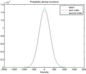
From Figure 6 can be seen that a second order Hermite polynomial is the best option. Figure 7 shows the plot for the data and a second order polynomial.

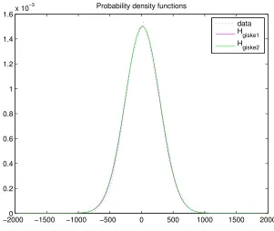
Her-−20000 −1500 −1000 −500 0 500 1000 1500 2000 0.2 0.4 0.6 0.8 1 1.2 1.4 1.6x 10

−3 _{Probability density functions}

data

H_giske1

H_giske2

Figure 7: A plot of two determined Hermite polynomials and the data

mite polynomial. Only the positive outliers are important, so only one second order polynomial is added.

Figure 8 shows two derived density functions and the probability density function of the data set. Equation (8) and (9) give the formulas for two estimated probability density functions. These functions are a sum of two Hermite polynomials and are found by trial-and-error.

Hgiske1(w) =

1 1.026197606 ·

*

0.001502e−(w3852−15)2 + 2·10−6e

−(w−750)2 3502

+

(8)

Hgiske2(w) =

1 1.035548931 ·

*

0.001502e−(w3752−15)2 + 10−10(20 + 9w2)·e

−w2

3602

+

(9)

The norms of the difference for both functions with the data are given by (10) and (11).

&data₋Hgiske1&1 = 0.0351 (10)

&data₋Hgiske2&1 = 0.0366 (11)

The best plot, the function with the smallest norm, is the density function Hgiske1. This function

esti-mates the probability density function of the data the best.

4.2 Correlation

−20000 −1500 −1000 −500 0 500 1000 1500 2000 0.2 0.4 0.6 0.8 1 1.2 1.4 1.6x 10

−3

Intensity

Probability density functions

data1 zero order second order

Figure 8: A plot of two determined Hermite polynomials

the correlation coefficient are calculated. The correlation coefficient between x and zis defined as

ρx,z := E[(

x₋E(x))(z₋E(z))]

σxσz (12)

= E[(x−x¯)(z−z¯)]

σxσz (13)

' (N

i=1(xi−x¯)(z−z¯)

(N₋1)sxsz

(14)

' (N

i=1(xi−x¯)(z−x¯)

(N₋1)s2

x

. (15)

Equation (15) is the one programmed in Matlab. We calculate the correlation coefficient between two pixels in one data set. Therefore the means for x and z are the same. For pixel z we take a neighbor

of pixel x and this is repeated for the eight (direct) neighors. The location of the eight neighbors are

given in Table 1, where x has the general location (g, h). The edges of the image have less neighbors

therefore they are not taken along.

The correlation coefficient for the neighbor one slice up or down is calculated similar. This coefficient is the correlation for pixelx with the same pixel one slice up or down (neighborsst+1 andst−1,

Figure 9: Plot of the matrix of the phantom study

neighbor location direction

z1 (g-1,h) north

z2 (g-1,h+1) north-east

z3 (g,h+1) east

z4 (g+1,h+1) south-east

z5 (g+1,h) south

z6 (g+1,h-1) south-west

z7 (g,h-1) west

z8 (g-1,h-1) north-west

Table 1: Correlation for eight neighbors

The reason for the smaller value of the diagonal neighbor is the distance between the pixels. The pixel-spacing (pspace) is 4,07283mm, which results is a distance between a pixel and his diagonal neighbor of

√

2·pspace. Therefore the correlation coefficient for the diagonal pixel is smaller. The distance between

two slices, the slice location, is 3 mm. This explains the larger coefficient value for the upper (and lower) slice-correlation coefficient.

As can be seen in the plot of the intensity matrix of the phantom data (Figure 9) the original data ma-trix has correlated noise. For instance, pixels with a high intensity are clustered. From the correlation coefficients it can similarly be concluded that the data is correlated.

4.3 Covariance matrix

neighbor correlation

z1 0,4134

z2 0,2624 z3 0,4443 z4 0,2630 z5 0,4135 z6 0,2624 z7 0,4443 z8 0,2630 st−1 0,5556 st+1 0,5596

Table 2: Correlation for ten neighbors

z8 z1 z2

z7 x z3

z6 z5 z4

Table 3: First round of neighbors

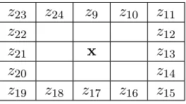
z23 z24 z9 z10 z11

z22 z12

z21 x z13

z20 z14

z19 z18 z17 z16 z15

Table 4: Second round of neighbors

set. From a covariance matrix it is possible to examine which pixels are correlated, in combination with the knowledge of the position of the pixels. The equation for the covariance is

cov(x, z) := E[(x−E(x))(z−E(z))] (16)

= _E[(x₋µx)(z−µz)] (17)

= E(xz)₋E(x)E(z) (18)

= ρx,z·σ2x (19)

Normally the covariance between two vectors or inside a vector is calculated. In this situation the covariance of a matrix is necessary. Therefore the size of the covariance matrix becomes much larger. For each point of the data set a covariance vector must be derived. All these covariance vectors will be combined into one large covariance matrix R.

Table 2 show that there is a correlation between pixelxand its vertical neighborz. For instance, if pixel x has position (1,1) in the data matrix then there exists a correlation with pixel z in the matrix with

position (26,1) in the matrix. In the first covariance vector of pointx with (1,1) this means a value on

position 1 and 26. The data set in our situation has the size 25×25, which means 625 pixels and that

625 covariance vectors have to be determined. These vectors are also correlated with each other. To simplify the filling of the covariance matrixR, we choose to use another approach. Covariance matrix R is split up in blocks. These blocks describe a covariance matrix for each row with a certain row.

describes the covariance between two rows.

R=σ2      

R1,1 R1,2 · · · R1,m

R2,1 R2,2 ... ...

... ... ... ...

Rn,1 · · · · · · Rn,m

     .

The variable n indicates the row and m indicates the column. For a 4_×4 matrix, the covariance

matrix is of the form

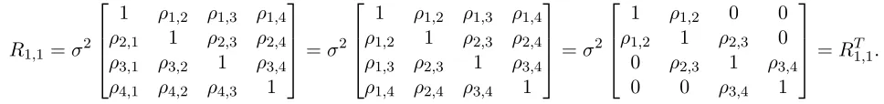
R1,1 =σ2    

1 ρ1,2 ρ1,3 ρ1,4 ρ2,1 1 ρ2,3 ρ2,4 ρ3,1 ρ3,2 1 ρ3,4 ρ4,1 ρ4,2 ρ4,3 1

   =σ2

   

1 ρ1,2 ρ1,3 ρ1,4 ρ1,2 1 ρ2,3 ρ2,4 ρ1,3 ρ2,3 1 ρ3,4 ρ1,4 ρ2,4 ρ3,4 1

   =σ2

   

1 ρ1,2 0 0 ρ1,2 1 ρ2,3 0

0 ρ2,3 1 ρ3,4

0 0 ρ3,4 1

  

=R1T,1.

The first observation is that the covariance of any pixel x with itself is the estimated variance (σ2_).

Secondly the correlation between pixels 1 and 2 (ρ1,2) is the same as the correlation coefficientρ2,1, see

Table 2. So this explains the first matrix operation.

The correlation between pixelx and its nth _{neighbors, for n >1, are calculated. These values become}

smaller as ngets larger. Therefore we assume that that there is no correlation between a pixel and its nth neighbor, forn >1. The main diagonal of the big covariance matrixR has the covariance matrices R1,1· · ·Rn,n, withn as the row indicator.

The upper and lower diagonal of matrixR represent the covariance matrices between rows. As shown

in the correlation-table, Table 2, there is correlation between the pixels on rowtandt+ 1. This matrix Rs of the same size (4×4) looks like,

Rs=σ2

   

ρs 0 0 0

0 ρs 0 0

0 0 ρs 0

0 0 0 ρs

   =RTs.

The resulting covariance matrix R is of the form

R=σ2    

R1,1 Rs 0 0

Rs R2,2 Rs 0

0 Rs R3,3 Rs

0 0 Rs R4,4

   =RT.

The size of this matrix R is 16×16. If the concept data matrix has a size of n×m, the covariance

matrix becomes (n·m)×(n·m). The main diagonal matrices are of sizem×m and that fornrows.

The data set of the PET data has a size of 25×25 so the covariance matrix is 625×625. A

co-variance matrix possesses some properties, among others it is symmetric and positive-semidefinite. The first property (M =MT_{) is easy to check since the sub-covariance matrix (R}

s) of the upper and lower

diagonal are the same and symmetric. The covariance on the main diagonal is symmetric because of equal correlation coefficients for the horizontal neighbors. For this reason the covariance matrix R is

The second property (positive semi-definiteness) is more difficult to check but important. A matrix

M ∈Cn×n _{is positive semi-definite ifx}∗_{M x≥0 for all x∈C}n_{, or for allx∈R}n _{ifM is a real matrix.}

Another way of checking positive semi-definiteness is showing that all the sub-determinants of the ma-trix are nonnegative. All 625 sub-determinants are calculated and the result is that the mama-trix is not positive semi-definite while a covariance matrix is positive semi-definite by definition. To conclude, our choice of covariance matrix is not correct and needs to be adjusted.

There are several explanations for the incorrectness of the proposed covariance matrix R. One

pos-sibility is that the matrix is filled incorrectly but this seems not be the case. The first solution we tried was to add more correlation coefficients because the covariance between pixelxand its direct horizontal

neighbor is approximately 34506 (ρ1,2·σ2), which is large.

The covariance for pixel x and its second horizontal neighborz13 is said to be zero, because the

calcu-lated correlation coefficient is small. However because of the large variance the covariance (ρ_·σ2) is too

large to neglect, so the covariance of the second (horizontal) neighbors are added. These neighbors are pixelsz13 and z21 respectively, see Table 4.

The other correlations (and covariances) are observed and they are too large to neglect as well. Thus the covariance of the diagonal neighbor (pixel z2 orz4) and the second vertical neighbors (pixelz9 andz17)

are added. The result of these operations is that the covariance matrix is finally positive semi-definite. The final covariance matrix R, after all additions, is of the form

R=σ2    

R1,1 Rs Rs2 0

Rs R2,2 Rs Rs2

Rs2 Rs R3,3 Rs

0 Rs2 Rs R4,4    .

The sub covariance matrices are of the following form

R1,1=σ2    

1 ρ1,2 ρ1,3 0 ρ1,2 1 ρ2,3 ρ2,4 ρ1,3 ρ2,3 1 ρ3,4

0 ρ2,4 ρ3,4 1   

, Rs=σ2

   

ρs ρd 0 0

ρd ρs ρd 0

0 ρd ρs ρd

0 0 ρd ρs

  

, Rs2 =σ2    

ρs2 0 0 0

0 ρs2 0 0

0 0 ρs2 0

0 0 0 ρs2

   ,

with ρs the degree of correlation between a pixel and his direct (horizontal or vertical) neighbor (pixel

z1 or z3). The correlation coefficient between a pixel and his second direct neighbor is given by ρs2

(= cov(x, z9) = cov(x, z17)). The variable ρd gives the correlation coefficient between a pixel and a

diagonal (upper or lower) neighbor (pixel z2 orz4).

4.4 Random values from the distribution

Now we have more information about the noise and so with the determined distribution of the noise it is possible to perform experiments. These experiments have the purpose to simulate the reality and hopefully give an idea how to distinguish suspicious pixels from normal pixels.

to use a sum of two Hermite polynomials to appoint deviant tissue. Moreover the two added Hermite polynomials have to be estimated and adapted for every patient.

The covariance matrix R is required for generating random values of a correlated normal

distribu-tion. In mathematical terms such a distribution is called a multivariate normal distribution [3, 10, 20]. This is the generalisation of a one-dimensional (univariate) normal distribution to higher dimensions. Matlab can generate random values from a multivariate normal distribution. The determined covari-ance matrix is an input, together with a zero vector ¯x, for generating a correlated sequence. After

the simulations it is (hopefully) possible to have a criterion for excluding noise from pixels with some deviation. The latter is probably suspicious tissue.

The covariance matrix has the size 625×625 and the zero vector ¯x has 625 elements. The

result-ing multivariate vector has 625 elements and can be reshaped to a 25×25 simulation matrix with

correlated elements. Figure 11 shows the intensity matrix of the simulation matrix whereas in Figure 10 it is shown how an uncorrelated data set looks like. It can be seen that a correlated data set should be simulated instead of a uncorrelated (and simpler) data set, see Figure 9. Uncorrelated noise shows no clustering of points, while Figure 9 (an actual PET data-image) and 11 show clustering of high intensity points.

Figure 10: Uncorrelated noise Figure 11: Correlated noise

5

Simulations

The random values based on the multivariate distribution generated in Chapter 4 are used for simulations where the goal is to simulate a real situation. The simulation matrix will be influenced artifically by increasing one pixel. We refer to this pixel as the increased pixel. A to-be-designed algorithm has the task to detect the increased pixel. In our simulations we know the location of the increased pixel. For this reason it is possible to test the performance of the algorithm.

5.1 Determining an outlier

A pixel in the data set is called an outlier if its intensity is above a certain value. This limit value,

vlimit, is a constant number for a (normal) distribution.

Usually the number of outliers of a data set is defined as a percentage. In Figure 12, it can be seen that for a normal distribution approximately 95% of the values lie within two standard deviations from the mean. This criterion is known as the empirical rule.

Figure 12: Empirical rule of normal distribution [5]

With the error-function [6] corresponding to the normal distribution it is possible to calculate the interval that contains any percentage of the data. For the mean and variance of the nosie, estimated from the orginal PET image, the limit value for 5% outliers is 475. (For 10% outliers the limit is 370 and for 1% it is 672.) The 95% interval contains positive outliers only and is called one sided, i.e.

2 vlimit

−∞

f(x)dx= 0.95.

5.2 Distance

described before a high intensity does not automatically mean that it is suspicious. It has been shown that pixels are correlated with each other. The hypothesis is that a suspicious pixel distinguishes itself from an outlier by a smaller correlation with its neighbors although it is hard to calculate this correlation. Therefore the difference between an outlier and a suspicious pixel could be found by looking to the differences in distance.

The distance (d) is the difference between the intensity of a pixel and one of its neighbors, see (20). The

average distance d is the sum of all distances, for all h neighbors, divided by the number of neighbors

for pixel i.

d := |x−z| (20)

di := 1

h

h

!

k=1

|xi−zk| (21)

The neighbors of the outlier are probably also relatively high because of the correlation between these pixels. Therefore the hypothesis is that the average distance for an outlier (do) will be smaller than the

average distance for an increased pixel (dp).

5.3 One increased pixel

A possible way of distinguishing a suspicious pixel from an outlier is described in Subsection 5.2. For simulation of a PET image one pixel in the data set will be increased. This increased pixel can be seen as a suspicious pixel in reality. The intensity of the increased pixel is raised to a value abovevlimit.

The methodology of the simulations is to identify all outliers, including the increased pixel, and to calculate all distances. The first round takes all eight direct neighbors. The second round consists of the sixteen neighborsz9−z24.

Equations (22) and (23) give the formula for the distance for the first and second neighborhood round.

dr1,i := 1₈

8 !

k=1

|xi−zk| (22)

dr2,i := ₁₆1

24 !

k=9

|xi−zk| (23)

The results of the two rounds are shown in Table 5 for different percentage outliers. It turns out that the average distance between an outlier and its direct eight neighbors is twice as small as the average distance for the increased pixel. This ratio is smaller for the second round.

This means that the results of the first round are sufficient to distinguish an outlier from the increased pixel. The second round is not necessary anymore. As shown before these neighbors have less corre-lation with the outlier because of the pixel space (pspace). The correlation between a pixel and itsnth

neighbor decreases rapidly for n larger than one which means that the influence of the noise is larger

than the influence of the correlation between pixels. Also the diagonal neighbors may not have a sig-nificant influence because of the pixel distancepspace. Therefore only the direct neighbors (z1, z3, z5, z7)

are taken into account. Table 6 gives the definition of the neighbors and their corresponding direct neighbors from Table 3.

1% dr1 dr2

outlier 518 759 pixel 1002 1008

5%

outlier 414 594

pixel 714 711

10%

outlier 365 513

pixel 558 562

Table 5: Different intensity values for two rounds of neighbors and different percentage outliers

Pixel Location

n1 z1

n2 z3

n3 z5

n4 z7

Table 6: Four direct neighbors and their location

the squared distance is the possibility to say something about the theoretical background. It is difficult to say something about the expected value for the absolute distance, while the expected value for the squared distance has some similarities with a (co)variance or standard deviation.

For the comparison of the outliers with the increased pixel, the distance between a pixel and its neigh-bors is calculated. Table 7 shows the results for these calculations. The formula for do and dp is the

same. The only difference is the pixelx. Fordothis is an outlier and in the case ofdp it is the increased

pixel.

For the sake of simplicity Equation (25) is used to calculate the squared distance. The average squared distance is determined by adding all squared values (for all outliers) and dividing by the number of outliers. The average distance for the increased pixel with its neighbors is just the value calculated by Equation (25) since there is just one increased pixel. If there are more increased pixels, the mean has to be taken for determining the average distance.

di = 1₄

4 !

k=1

|xi−nk| (24)

di,2 = 1₄ 4 !

k=1

|xi−nk|2 (25)

The increased pixel has an intensity of 1.5·vlimit, with vlimit the limit value as explained in

Subsec-tion 5.1. As given before the limit value for 1% outlier is 370 and 475 for 5%.

This value intensity value is chosen arbitrary such that the pixel is larger than vlimit but smaller than

β = 5% β= 1%

Outlier Pixel Outlier Pixel

d 368 711 459 1010

d2 _{189391 588245 266465 1083509}

Table 7: Difference in distance for two percentage outliers

A confidence interval is used to indicate the reliability of an estimator. The interval is observed, which means that the values are calculated from observations. For a 95% confidence interval in 95% of the cases the average (squared) distance will be between the calculated endpoints. However in 5% of the cases, it will not be.

Every confidence interval is of the following form,

[ ¯d₋c√·s n,d¯+

c_·s √

n] (26)

withc being a value from the cumulative standard normal distribution function.

The variable α is a fixed number and gives the change (in percentage) that the average distance will

not be between the endpoints. The choice of the number zis described below.

P(₋z_≤X_≤z) = 1₋α _⇔

P(|X|> z) = α (27)

P(−z < X) = P(X > z) = 1

2α. (28)

Because of the symmetry of the distribution around 0, we get

P(X ≤z) = 1−1₂α. (29)

This construction is necessary because of the values in the cumulative standard normal distribution table [23].

φ(c) =P(Z_≤c).

The variable c gets the value φ−1(z), with z = 1−12α. For α = 0.05 we havec = 1.96. The value of s is the estimated standard deviation calculated by Equation (4) on page 22. ¯dis the average of the

distance and nis the number of simulations used for the confidence interval.

Table 8 shows 95% confidence intervals for the average distance and the squared distance, both for an outlier and an increased pixel.

β = 5% Outlier Pixel β = 1% Outlier Pixel

d [367 ; 370] [704 ; 719] [456 ; 462] [1003 ; 1018]

d2 [188204 ; 190578] [576482 ; 600008] [263347 ; 269583] [1067289 ; 1099728]

As it can be seen, the confidence intervals for the outlier and pixel do not overlap. This is nice because the confidence intervals are used for determining whether a pixel is noise or suspicious tissue.

6

Validation of the model

0 1 2 3 4 5 6 7 8 9

x 105 0 0.5 1 1.5 2 2.5 3 3.5 4

4.5x 10

−5 _{Frequency plot of 10% outliers}

distance d

i,2 Frequency (# * tot

−

1 )

outlier pixel

Figure 13: Histogram of the squared distance for 10% outliers

Figure 13 shows the frequency plots of the distance of the outlier and of the increased pixel where the distance is calculated by (25). This figure shows a large overlap between the support of the two plots. However the confidence intervals, as defined in (26), for an outlier and an increased pixel show no overlap and thus some questions regarding the credibility of the histogram arise. What is the expected value for the distance of an outlier and increased pixel? Will these theoretical values for the mean distance and variance of the distance for the outlier and pixel agree with the values resulting from the simulations?

In the next subsection we reproduce the formulas for the expectation and the variance of the increased pixel. These derivations are relatively simple because an increased pixel is fixed and hence it does not have a probability distribution. It is harder to derive the theoretical values for the outliers. The derivatioins shown here are rather short, the complete deduction can be found in Appendix B, on page 63.

6.1 Theoretical values of an increased pixel

The formula of the expected value for the distance between an increased pixel and its neighbors is explained here. Thus we calculate

E 3 1 4 4 ! b=1

(y−xb)2

4

wherexb is a neighbor of y, the increased pixel.

The expectation of a sum is the sum of the expectations, therefore the formula can be written as

E 3 1 4 4 ! b=1

(y₋xb)2

4 = 1 4 4 ! b=1

E[(y₋xb)2] (31)

For each neighborxbthe expectation is the same and the correlation between the increased pixely(with

constant value) and its neighbor xb is known.

E[(y₋xb)2] = E[(y−µ+µ−xb)2], with E(xb) =µ (32)

= _E[((y₋µ)₋(xb−µ))2] (33)

= _E[(y−µ)2−2(y−µ)(xb−µ) + (xb−µ)2] (34)

= (y−µ)2+σ2_x (35)

= y2+σ_x2, (36)

where we used that µ= 0, see page 31. The variable σ_x2 is the variance of the noise, i.e. the standard

deviation from (4) squared.

Deriving the variance of the increased pixel is a little harder. The equations become very large if all elements are described. For this reason, only the variance of one neighbor is described.

var(W) = 1

16var

5 ₄ !

b=1

(y₋xb)2

6

, since var(ax) =a2var(x) for a_∈R (37)

= 1

16

4 !

b=1

var(Wb) + 2

!

b<j

cov(Wb, Wj), withWb = (y−xb)2. (38)

First the derivation of the variance for each neighbor is explained shortly. By (66), we have

var(Wb) = E[(y−xb)4]−(E[(y−xb)2])2 (39)

The expectation of the fourth moment is not that easy. Using E(xb) = 0 and (98) we find

E[(y−xb)4] = y4+ 6y2σx2+ 3σ4x (40)

Now we have derived the fourth moment. The expectation of (y−xb)2 is shown previously in (36), so

the square of it is also known. The formula for the variance is found by combining (66) with the results above.

var(Wb) = 2σ4x+ 4y2σ2x (41)

The equation for the covariance of an increased pixel is derived by using (71). cov

b<j(Wb, Wj) := E[WbWj]−E[Wb]E[Wj],

E[WbWj] = y4+ 2σx2y2+σx4+ρb,j(4y2+ 2ρb,j),

cov

b<j(xb, xj) = ρb,j (42)

E[Wb]E[Wj] = E[Wb]2, forb= 1,2,3,4

cov

b<j(Wb, Wj) = σ

2

xρb,j(4y2+ 2σx2ρb,j) for b < j (43)

The last step is summing up all the variances and covariances, see Equation (38), and hence var(W) is

6.2 Theoretical values of an outlier

An outlier comes from the same data set as the increased pixel, henceforth it is assumed that the set with outliers is distributed normally. The steps shown above are also used for deriving the theoretical values for an outlier. After some extensive calculations the following formula is derived for the expectation of the distribution of an outlier:

E[(x₋xb)2] =σ2(1−ρv−ρh), (44)

withρv andρh the correlation coefficient for a vertical and horizontal neighbor, respectively. Pixelx is

an outlier and xb is a neighbor.

Only the theoretical values do not match with the results obtained from the simulations. The assumption that the outliers are distributed normally is not correct. The reason is that there is a condition for determining the outlier point x. This condition states that x is above the limit value (vlimit). This

condition must be taken into account when performing the calculations and therefore the distribution of x changes into a conditional distribution.

Point X is an pixel and point T is a neighbor and say X and T are distributed normally. The joint

probability density function of a multivariate normal distribution is given by (45)

fX(x) =

1 (2π)k_|Σ|12

e−12(x−µ)TΣ−1(x−µ), (45)

with X=* X

T +

. SinceX andT have the same expectation and variance, we find

fX,T(x, t) =

1

2πσ27_1−ρ2e

− 1

2(1−ρ2)σ2[(x−µ)2+(t−µ)2−2ρ(x−µ)(t−µ)]_, (46)

where ρ is the correlation coefficient between pointX and T.

Given this joint probability density function we derive a formula for the conditional probability density function

f_X,T|X>a(x, t), (47)

where X is an outlier and T is a neighbor.

The cumulative conditional density function for the outlier case is given by

FX,T|X>a(x, t) = P(X ≤x, T ≤t|X > a) (48)

= 1

P(X > a)·P(a≤X ≤x, T ≤t) for x > a (49)

= F(x, t)−F(a, t)

1−F(a) , (50)

where F(a) = P(X _≤a) = 1 σ√2π

2 a

−∞

e−12(

x−µ

σ )2dx (51)

with P(X≤x) = 2 x

−∞

fX(x)dX (52)

Where Bayes Rule [23] is used to go from (48) to (49).

By using

F_X,T|X>a(x, t) = 2 x

−∞

2 t

−∞

f_X,T|X>a(ϕ,τ)dϕdτ, (54)

we see that the conditional probability density function becomes

f_X,T|X>a(x, t) = ∂ 2

∂x∂tFX,T|X>a(x, t) (55)

= 1

1−F(a)fX,T(x, t) forx > a,−∞< t <∞, (56)

withfX,T given by (46).

For a standard normal distribution, the expectation of X2 can be derived as

E[X2] = 2 _∞

−∞

x2fX(x)dx with the probability functionfX(x).

Thus the expected value of the distance of an outlier is given by (58).

E[(X−T)2|X > a] = 2 _∞

a

2 _∞

−∞

(x−t)2fX,T|X>a(x, t)dt dx (57)

= 1

1−F(a) 2 _∞

a

2 _∞

−∞

(x₋t)2fX,T(x, t)dt dx (58)

Figure 14 shows the two dimensional plot for the conditional probability density function from (56).

6.3 Conditional variance

The theoretical value for the variance of the outlier is derived in the same way [4].

var(X_|Y) = E[(X₋E[X_|Y])2_|Y] (59)

= _E[X2_|Y]₋(E[X_|Y])2 (60)

For the variance of the outlier the following equation can be used

var((X₋T)2_|X > a) = E[((X₋T)2)2_|X > a]₋(E[(X₋T)2_|X > a])2 (61)

= _E[(X−T)4|X > a]−(E[(X−T)2|X > a])2 (62)

The first part of (62) can be derived by (58) with (x−t)4 instead of (x−t)2. The second part of the