Inventory Model in a CVRP Distribution Network with Uniformly Distributed Demand

www.editada.org

Informatics, 11(2), May-Aug 2020, 75-85. ISSN: 2007-1558.

________________________________________________________________________________

Editorial Académica Dragón Azteca (EDITADA.ORG)

Inventory Model in a CVRP Distribution Network with Uniformly Distributed Demand

Lucía Cazabal-Valencia, Santiago-Omar Caballero-Morales, José-Luís Martínez-Flores, Damián-Emilio Gibaja-Romero

Universidad Popular Autónoma del Estado de Puebla A.C., Postgraduate Department of Logistics and Supply Chain Management, 17 Sur 901, Barrio de Santiago, 72410, Puebla, México

[email protected], [email protected], [email protected], [email protected]

Abstract. At the present time, business and industrial organizations are given the task of good planning when determining any type of acquisition for their services. That is, identify and evaluate the different options of provision of inventory that allow the company to maintain and improve its offer. Within this evaluation, it can be noticed that the decision of the management and administration of resources, involves the problem of distribution (goods and services), being also of great importance within the supply chain. In this way, in this paper, we analyze the Capacitated Vehicle Routing Problem with ellipsoidal distances, which includes an inventory model with uniformly distributed demands, so that inventory costs and distances are minimized. With this contribution, the way to minimize total costs in a distribution period can be refined. For validation, computational evaluations obtained from the mathematical model and backed by the software are presented (LINGO 18.0 - MATLAB).

Keywords: CVRP, uniform demand, newsvendor, ellipsoid

Article Info

Received Jul 30, 2019 Accepted Dec 11, 2019

1

Introduction

From an economic, industrial, financial and capital flow perspective, the problem of inventories has always been present, and this arises when it is realized that the costs of maintaining, incurring shortages and replenishing, associated with a particular product that is required for production, commercialization or consumption, they are found and, consequently, there is an optimum (in this case, a minimum cost) that must be located [1].

Inventory management is the process in charge of ensuring the number of adequate products in the organization, in such a way that the manufacturing and distribution operations do not stop, fulfilling the promises of delivery of products to customers. However, maintaining these inventories in organizations represents considerable costs, since for this activity it is required: capital investments in the goods, space to store them, personnel for their administration and care and technological and energy resources are required for their maintenance among others [2].

All firms (including JIT operations) maintain an inventory provision for the following reasons [3]:  Maintain independence in operations.

 Adjust to the variation of product demand.  Allow flexibility in production scheduling.

 Provide a safeguard for the variation in the delivery time of raw materials.  Take advantage of the size of the economical purchase order.

Each of the reasons mentioned takes great importance, since when making any decision that affects the size of the inventory they generate undesirable costs [4]:

76

 Costs of insufficient supply in the short run

In this paper, the inventory of a certain item that is reviewed every fixed time interval will be addressed; that is, the order size varies with the behavior of the demand.

It is beneficial for any company to use logistics strategies, in terms of obtaining general corporate skills, since one of the most important characteristics of the logistics strategies must be to find a way to minimize the total cost in the distribution period, that is; achieve minimize distribution costs by determining the best route of the vehicle while serving the customer [5].

As already mentioned, maintaining a high number of inventories with which the customer is satisfied, but which incurs high costs is a dilemma for any organization, now if we add the costs for distribution of this matter this implies, even more, the management of a successful decision. For this reason, the Capacitated Vehicle Routing Problem (CVRP) is analyzed, which can be described in a simple way, such as a fleet of vehicles with homogeneous capacities that have to satisfy the uniformly distributed demand of a group of customers through a set of routes that start and end in a common center and that have as an objective, minimize the cost of the route that in turn is implied by the total coverage distance.

In section 2, a brief analysis of the single-period inventories with uniformly distributed demands will be addressed, as well as the CVRP proposed with an ellipsoidal geodetic length for distance minimization. Later, the influence and/or significance of the optimal quantities to be ordered in the Capacitated Vehicle Routing Problem will be seen with the customer demand distributed uniformly.

2

Technical Framework

2.1 Inventories: Single Period Problem

Liao et al. [6] they mention that the inventory and the possession of products in any distribution center are a subject of great importance in the supply chain and in their contribution they consider cross-docking as an efficient method to control the flow of inventory.

Within the stock management literature, the problem of newsvendor or also known as Single Period Problem (SPP) is mentioned, which consists of finding the quantity of a product that maximizes the expected profit under a random demand (probabilistic). The SPP model assumes that, if any inventory remains at the end of the period, a discount is used to sell it or liquidated, if the quantity of the order is less than the demand made, some profits are renounced [7].

The investigations on the problem newsvendor have followed two approaches for their solution:  Minimize the expected costs of overestimating and underestimating demand.

 Maximize the expected benefit.

While this problem is used in many real-life situations, some of the most prominent are mentioned [2] [7]:  Perishable or expired items.

 Articles at the end of their life cycle.

 Fashion items, sports and in general those sold by campaigns.  Design and management of the adequate capacity of an installation.  Evaluation of advanced reservation of orders in airline and hotel services.

11(2) 2020, 75-85.

77

The optimal quantity of order is the one that covers the proportion of the demand up to a Critical Relationship (CR) that oscillates between 0 and 1; this can represent as:

𝐶𝑅 = 𝑐𝑠

𝑐𝑠+ 𝑐𝑒 Where:

𝑐𝑠= 𝑐𝑜𝑠𝑡 𝑜𝑓 𝑠ℎ𝑜𝑟𝑡𝑎𝑔𝑒

𝑐𝑒= 𝑐𝑜𝑠𝑡 𝑜𝑓 𝑒𝑥𝑐𝑒𝑠𝑠

(1)

The parameters that impact the cost of the shortage and the cost of the excess are the sale price, the cost, the recovery value and the shortage penalty, all at the unit level. Using these parameters, we can derive the cost of the shortage and the cost of the excess as:

𝑐𝑠= 𝑝 − 𝑐 + 𝐵 y 𝑐𝑒= 𝑐 − 𝑔. Where:

𝑐 = 𝑐𝑜𝑠𝑡 𝑝 = 𝑠𝑒𝑙𝑙𝑖𝑛𝑔 𝑝𝑟𝑖𝑐𝑒 𝐵 = 𝑠ℎ𝑜𝑟𝑡𝑎𝑔𝑒 𝑝𝑒𝑛𝑎𝑙𝑡𝑦

𝑔 = 𝑠𝑎𝑙𝑣𝑎𝑔𝑒 𝑣𝑎𝑙𝑢𝑒

When we replace in equation (1) and assuming that there is no penalty for shortage, you have to 𝐶𝑅 =𝑝−𝑐

𝑝−𝑔. Keep in mind that, if there is no recovery value, this is further simplified:

𝐶𝑅 =𝑝 − 𝑐 𝑝

(2)

Since CR represents the accumulated demand up to the optimal order quantity, it follows that:

𝐶𝑅 = 𝐶𝐷𝐹(𝑄∗₎

𝑄∗_{= 𝐶𝐷𝐹}−1_(𝐶𝑅)

Where:

𝑄∗_{= 𝑂𝑝𝑡𝑖𝑚𝑎𝑙 𝑂𝑟𝑑𝑒𝑟 𝑄𝑢𝑎𝑛𝑡𝑖𝑡𝑦}

(3)

As already mentioned, the objective of Newsvendor is to maximize profits from a fixed offer while the demand is uncertain or to minimize the expected costs of overestimating and underestimating the order. In this paper, we will focus on minimizing the expected costs. When using the Newsvendor model, we know that the values are stochastic. Therefore, we will calculate the expected cost by:

𝐸(𝑐) = 𝑐𝑄∗_{+ 𝐵𝐸(𝑠ℎ𝑜𝑟𝑡𝑎𝑔𝑒)}

₍₄₎

As:

∗_{, 𝑠𝑖 𝐷 ≥ 𝑄}∗

0, 𝑠𝑖 𝐷 < 𝑄∗

(5)

So:

𝑥=𝐷

(6)

Take into account that 𝐸(𝑠ℎ𝑜𝑟𝑡𝑎𝑔𝑒) determines the number of insufficient units.

2.2 Uniform distribution

A uniform random variable is used to model the behavior of a continuous random variable whose values are uniform or exactly distributed in a given interval [𝑎, 𝑏] [9]. The probability density function of the continuous uniform distribution is given by:

𝑓(𝑥) = { 1

𝑏 − 𝑎 𝑠𝑖 𝑎 ≤ 𝑥 ≤ 𝑏

0 𝑝𝑎𝑟𝑎 𝑥 < 𝑎 𝑜 𝑥 > 𝑏

(7)

78

Now, if the demand follows a uniform distribution, it is obtained from (3) that the optimal quantity to be ordered is given by:

𝑄∗_{= 𝐶𝑅(𝑏 − 𝑎) + (𝑎)} Where:

𝑎 = 𝑙𝑜𝑤𝑒𝑟 𝑏𝑜𝑢𝑛𝑑 𝑜𝑓 𝑑𝑒𝑚𝑎𝑛𝑑 𝑏 = 𝑢𝑝𝑝𝑒𝑟 𝑏𝑜𝑢𝑛𝑑 𝑜𝑓 𝑑𝑒𝑚𝑎𝑛𝑑

(8)

2.3 Capacitated Vehicle Routing Problem

The Capacitated Vehicle Routing Problem (CVRP) is an evolution of the Vehicle Routing Problem (VRP), which in turn has origins from the Traveling Salesman Problem (TSP) raised in 1956. The main objective of the TSP is to find the best possible route from different approaches (already be a process with some specific sequence or a logistic distribution) with criteria of economy in distances or costs [10].

The VRP type problems are the most frequent in combinatorial optimization, and most of them belong to the NP-Hard class. Rocha et al. [11] perform a revision of the taxonomy of these problems from the conceptual point of view of mathematical formulation and of the solution methods used. It should be mentioned that a formulation of the VRP type can include a large number of variables and various parameters, since this raises the search for the optimal solution with different restrictions such as; number of vehicles, capacity, places of destination, customer demand, among other.

For the CVRP the outstanding variable is the quantity of product, both for the demand of the customers and for the capacity of the vehicles. It is worth mentioning that the capacity restriction for vehicles is classified as a homogeneous and heterogeneous fleet. For the purposes of this study, vehicles with equal capabilities will be taken, that is; homogeneous fleets.

Before presenting the mathematical model of the CVRP it will be important to mention the characteristics that distinguish this problem [12]:

 Given a set of customers geographically distributed in a certain defined area, there will be a point that will deliver a single product to all customers.

 Each customer has a constant demand for a known product, and must be visited by a fleet of identical vehicles with limited capacity.

 The distance and / or cost between the customers and the point of supply is known.

 The vehicles are initially located in the warehouse where each of the routes starts, then they visit a subgroup of customers and finally return to the warehouse.

 The sum of the demands of customers who visit a vehicle must be equal to or less than the capacity of said vehicle.  Each client must be visited by a single-vehicle.

 It is assumed that the amount of product available in the deposit is equal to or greater than the sum of the demands of all customers.

 The capacity of all vehicles is greater than or equal to the sum of the demands of all customers, i.e., All customers will be satisfied in the totality of their demand.

 The cost of the route may depend on time, distance, fuel consumption or others, however, the purpose will always be to minimize it.

In consideration of the aforementioned characteristics, the mathematical model of the CVRP assumes the following form [13]:

𝑀𝑖𝑛 ∑ ∑ ∑ 𝑑𝑖𝑗 𝑥𝑖𝑗𝑘 𝑀

𝑘=0 𝑁

𝑗=0 𝑁

𝑖=0

(9)

𝑠. 𝑎. ∑ ∑ 𝑥𝑖𝑗𝑘 ≤ 𝑀 𝑖 = 0 𝑁

𝑗=𝑖 𝑀

𝑘=1

(10)

∑ ∑ 𝑥𝑖𝑗𝑘 = 1 ∀𝑖 ∈ [1, 𝑁] 𝑁

𝑗=0 𝑀

𝑘=1

11(2) 2020, 75-85.

79

∑ 𝑥𝑖𝑗𝑘= ∑ 𝑥𝑖𝑗𝑘 𝑁

𝑖=1

∀𝑘 ∈ [1, 𝑀], 𝑖 = 0

𝑁

𝑗=1

(12)

∑ ∑ 𝑝𝑖𝑥𝑖𝑗𝑘≤ 𝑃𝑘 𝑁

𝑗=0

∀𝑘 ∈ [1, 𝑀]

𝑁

𝑖=0

(13)

∑ ∑ 𝑥𝑖𝑗𝑘≤ |𝑆| − 1 |𝑆| ≥ 2, ∀𝑖, 𝑗 ∈ [1, 𝑁] 𝑁

𝑗=1 𝑁

𝑖=1

(14)

𝑥𝑖𝑗𝑘∈ {0,1} ∀𝑘 ∈ [1, 𝑀], ∀𝑖, 𝑗 ∈ [1, 𝑁]

(15)

The restriction (10) indicates that from the supply center must depart maximum M vehicles. Restrictions (11) and (12) ensure that one and only one vehicle visits and abandons each customer, forming a TSP for each route. Equation (13) restricts vehicular capacity in terms of weight. Subsequently, the restrictions (14) and (15) establish, respectively, the absence of disconnected sub-routes and the binary values for the decision variables.

The objective function (9) establishes the minimization of costs, which for our purpose will be determined from the geodesic distances between the clients and the supply center. In this case, for the calculation of all the geodesic distances between two points, the ellipsoidal distance proposed by Cazabal [14] is considered:

𝑑 = 𝑠12= 𝑏𝐴(𝜎 − ∆𝜎)

(16)

The geodetic distance 𝑠12 connects two points 𝐴 = (𝜑1, 𝜆1) and 𝐵 = (𝜑2, 𝜆2) with latitude and longitude, Figure 1 shows the geodesic arc delimited by AB, known as the inverse problem on an ellipsoid.

Figure 1. Geodetic distance AB over an ellipsoid (From Cazabal [11])

3

Evaluation of the model

80

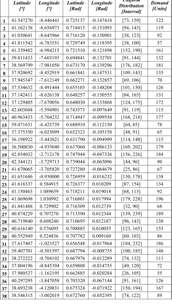
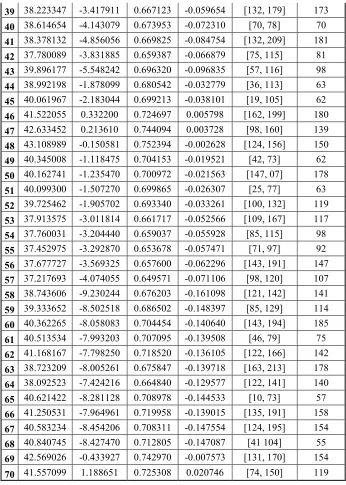
Table 1. Location of clients and respective demands

Latitude [°]

Longitude [°]

Latitude [Rad]

Longitude [Rad]

Uniform Distribution

[Interval]

Demand [Units]

1 41.547270 -8.446441 0.725137 -0.147418 [73, 159] 122 2 41.162138 -8.656973 0.718415 -0.151093 [94, 143] 119

3 41.030641 -8.645966 0.716120 -0.150901 [38, 123] 92 4 41.811542 -6.783551 0.729749 -0.118395 [38, 100] 57 5 41.339482 -6.984215 0.721510 -0.121898 [152, 190] 161 6 39.811433 -7.603193 0.694841 -0.132701 [91, 144] 132

7 38.569799 -7.981050 0.673170 -0.139296 [176, 182] 181 8 37.920692 -8.452919 0.661841 -0.147531 [109, 143] 135

9 37.945347 -7.612149 0.662271 -0.132857 [69, 106] 70

10 37.534632 -8.491444 0.655103 -0.148204 [101, 150] 126 11 37.142411 -8.626138 0.648257 -0.150555 [84, 165] 131

12 37.129405 -7.670056 0.648030 -0.133868 [124, 175] 172 13 42.603604 -5.594901 0.743573 -0.097649 [91, 119] 115 14 40.963433 -5.704232 0.714947 -0.099558 [168, 218] 177

15 39.471631 -6.425739 0.688910 -0.112150 [64, 85] 78 16 37.375350 -6.025099 0.652323 -0.105158 [48, 91] 65 17 36.198922 -5.443021 0.631790 -0.094999 [114, 148] 115

18 36.500830 -4.935040 0.637060 -0.086133 [169, 202] 179 19 42.854032 -2.712178 0.747944 -0.047336 [156, 226] 184 20 42.344121 -3.729713 0.739044 -0.065096 [44, 96] 90

21 41.670065 -3.705820 0.727280 -0.064679 [25, 86] 67 22 41.651686 -0.930000 0.726959 -0.016232 [130, 178] 138 23 41.618337 0.584915 0.726377 0.010209 [87, 154] 134

24 41.150463 1.089659 0.718211 0.019018 [68, 113] 92 25 41.069698 1.030992 0.716801 0.017994 [179, 228] 196

26 41.041488 0.729902 0.716309 0.012739 [32, 90] 68

27 40.874229 0.707270 0.713390 0.012344 [139, 239] 189 28 40.719840 0.698240 0.710695 0.012187 [96, 143] 138

29 40.616140 0.576095 0.708885 0.010055 [123, 165] 155

30 40.552949 0.524836 0.707782 0.009160 [60, 103] 86 31 37.617407 -1.023527 0.656548 -0.017864 [184, 232] 186

32 39.407701 -0.501597 0.687794 -0.008755 [100, 185] 148 33 38.272222 -0.704102 0.667976 -0.012289 [74, 132] 111 34 37.804196 -0.845394 0.659808 -0.014755 [49, 120] 72

35 37.980527 -1.162195 0.662885 -0.020284 [26, 105] 55 36 40.297295 -3.847058 0.703320 -0.067144 [91, 161] 126

37 38.693238 -4.120831 0.675324 -0.071922 [150, 194] 167

11(2) 2020, 75-85.

81

39 38.223347 -3.417911 0.667123 -0.059654 [132, 179] 173

40 38.614654 -4.143079 0.673953 -0.072310 [70, 78] 70 41 38.378132 -4.856056 0.669825 -0.084754 [132, 209] 181

42 37.780089 -3.831885 0.659387 -0.066879 [75, 115] 81

43 39.896177 -5.548242 0.696320 -0.096835 [57, 116] 98 44 38.992198 -1.878099 0.680542 -0.032779 [36, 113] 63

45 40.061967 -2.183044 0.699213 -0.038101 [19, 105] 62

46 41.522055 0.332200 0.724697 0.005798 [162, 199] 180 47 42.633452 0.213610 0.744094 0.003728 [98, 160] 139

48 43.108989 -0.150581 0.752394 -0.002628 [124, 156] 150 49 40.345008 -1.118475 0.704153 -0.019521 [42, 73] 62 50 40.162741 -1.235470 0.700972 -0.021563 [147, 07] 178

51 40.099300 -1.507270 0.699865 -0.026307 [25, 77] 63 52 39.725462 -1.905702 0.693340 -0.033261 [100, 132] 119 53 37.913575 -3.011814 0.661717 -0.052566 [109, 167] 117

54 37.760031 -3.204440 0.659037 -0.055928 [85, 115] 98 55 37.452975 -3.292870 0.653678 -0.057471 [71, 97] 92 56 37.677727 -3.569325 0.657600 -0.062296 [143, 191] 147

57 37.217693 -4.074055 0.649571 -0.071106 [98, 120] 107 58 38.743606 -9.230244 0.676203 -0.161098 [121, 142] 141 59 39.333652 -8.502518 0.686502 -0.148397 [85, 129] 114

60 40.362265 -8.058083 0.704454 -0.140640 [143, 194] 185 61 40.513534 -7.993203 0.707095 -0.139508 [46, 79] 75

62 41.168167 -7.798250 0.718520 -0.136105 [122, 166] 142

63 38.723209 -8.005261 0.675847 -0.139718 [163, 213] 178 64 38.092523 -7.424216 0.664840 -0.129577 [122, 141] 140

65 40.621422 -8.281128 0.708978 -0.144533 [10, 73] 57 66 41.250531 -7.964961 0.719958 -0.139015 [135, 191] 158 67 40.583234 -8.454206 0.708311 -0.147554 [124, 195] 154

68 40.840745 -8.427470 0.712805 -0.147087 [41 104] 55 69 42.569026 -0.433927 0.742970 -0.007573 [131, 170] 154 70 41.557099 1.188651 0.725308 0.020746 [74, 150] 119

The assumption is made to supply items with the specifications given in Table 2.

Table 2. Item data per unit

c Cost (purchase price) $ 320.00

p Selling price $ 500.00

82

It is necessary to emphasize again that the objective of the CVRP is to minimize the cost of the route, which in turn is implied by the total coverage distance. This distance is obtained considering the ellipsoid as the model for the surface of the Earth and with this making use of the geodetic distance (16).

3.1. Results

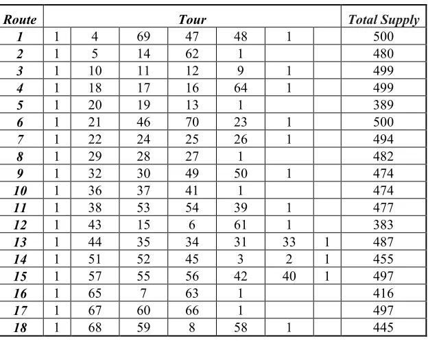
The tests were performed considering the location data of clients presented in Table 1 and Eq. 16 for the calculation of the distance matrix that is subsequently implemented in the CVRP model, which was used for the execution of the LINGO 18.0 Software. For all routes, vehicles with the same capacities were considered 𝑃𝑘 = 500, 𝑘 = 1, … ,18. Table 3 presents the 18 optimal routes with a total route of 210.7730 𝑘𝑚, the assigned tour is also presented respectively, as the amount of total product supplied.

Table 3. Optimal solution of the CVRP model with ellipsoidal distance

Route Tour Total Supply

1 1 4 69 47 48 1 500

2 1 5 14 62 1 480

3 1 10 11 12 9 1 499

4 1 18 17 16 64 1 499

5 1 20 19 13 1 389

6 1 21 46 70 23 1 500

7 1 22 24 25 26 1 494

8 1 29 28 27 1 482

9 1 32 30 49 50 1 474

10 1 36 37 41 1 474

11 1 38 53 54 39 1 477

12 1 43 15 6 61 1 383

13 1 44 35 34 31 33 1 487

14 1 51 52 45 3 2 1 455

15 1 57 55 56 42 40 1 497

16 1 65 7 63 1 416

17 1 67 60 66 1 497

18 1 68 59 8 58 1 445

For the execution of the newsvendor model, MatLab Software was used with (2), (4) and (8) and considering all the points except the 1, since from there all the routes start and end (Hamiltonian cycle, that is, it is not possible to form sub tours [15]). Table 4 shows the optimal quantities to be ordered and, in turn, the expected costs that these would generate.

Table 4. Optimal solution of the Newsvendor model

Points _{Order Quantity} (Q*) Optimal _{Expected cost} (E(c)) Points _{Order Quantity} (Q*) Optimal _{Expected cost} (E(c))

1 ---- ---- 36 117 $ 39,240.00

2 112 $ 37,140.00 37 166 $ 54,320.00

3 101 $ 32,320.00 38 92 $ 29,440.00

4 61 $ 19,520.00 39 149 $ 48,980.00

5 166 $ 53,120.00 40 73 $ 23,360.00

6 111 $ 36,820.00 41 160 $ 53,300.00

7 179 $ 57,280.00 42 90 $ 28,800.00

11(2) 2020, 75-85.

83

9 83 $ 26,560.00 44 64 $ 20,480.00

10 119 $ 39,380.00 45 50 $ 18,400.00

11 114 $ 38,580.00 46 176 $ 57,220.00

12 143 $ 47,060.00 47 121 $ 40,320.00

13 102 $ 33,240.00 48 136 $ 44,320.00

14 186 $ 59,520.00 49 54 $ 17,980.00

15 72 $ 23,540.00 50 169 $ 55,680.00

16 64 $ 21,580.00 51 44 $ 15,480.00

17 127 $ 40,640.00 52 112 $ 36,640.00

18 181 $ 57,920.00 53 130 $ 41,600.00

19 182 $ 60,040.00 54 96 $ 31,520.00

20 63 $ 21,560.00 55 81 $ 26,520.00

21 47 $ 16,740.00 56 161 $ 51,520.00

22 148 $ 47,360.00 57 106 $ 34,520.00

23 112 $ 37,540.00 58 129 $ 41,780.00

24 85 $ 28,300.00 59 101 $ 33,520.00

25 197 $ 63,040.00 60 162 $ 53,140.00

26 53 $ 18,560.00 61 58 $ 19,460.00

27 175 $ 58,800.00 62 138 $ 45,360.00

28 113 $ 37,460.00 63 181 $ 57,920.00

29 139 $ 45,480.00 64 129 $ 41,780.00

30 76 $ 25,420.00 65 33 $ 12,260.00

31 202 $ 64,640.00 66 156 $ 51,320.00

32 131 $ 44,220.00 67 150 $ 49,900.00

33 95 $ 32,000.00 68 64 $ 20,480.00

34 75 $ 24,000.00 69 146 $ 47,620.00

35 55 $ 19,700.00 70 102 $ 34,640.00

84

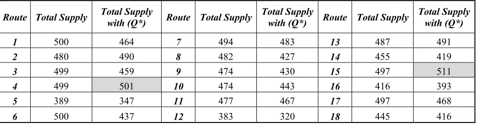
Table 5. Comparison of total supply - optimal quantity to order

Route Total Supply Total Supply _{with (Q*)} Route Total Supply Total Supply _{with (Q*)} Route Total Supply Total Supply _{with (Q*)}

1 500 464 7 494 483 13 487 491

2 480 490 8 482 427 14 455 419

3 499 459 9 474 430 15 497 511

4 499 501 10 474 443 16 416 393

5 389 347 11 477 467 17 497 468

6 500 437 12 383 320 18 445 416

It should be kept in mind that the costs to be ordered are independent of the costs for shipping or distribution, for this reason, the optimal routes are sought. The benefit of performing the CVRP analysis with a periodic inventory model and with uniformly distributed demands is to identify the agreement that exists between them, in such a way that costs and distances are minimized. Despite having a set of random variables (demands) that are distributed uniformly, it can be noted that their behavior does not differ significantly.

4. Conclusions

When facing economic-administrative decisions, the objective of every company is to maintain an acceptable service when minimizing the costs of operation, maintenance of inventory and transportation. Thus, in this article, we have presented the importance of the CVRP in distribution networks with a focus on inventory management and not only in terms of its solution techniques and taxonomy.

The CVRP with a periodic inventory analysis presents satisfactory results with 18 optimal routes that achieve the minimization of distances between 70 clients that must be satisfied, with a geodesic on an ellipsoidal surface, which resembles the most real form of the Earth.

When solving this problem, the problem of cost and service was attacked. That is, the transportation cost is reduced when distances are minimized and, on the other hand, by knowing the optimal quantity to be ordered, the cost to order is reduced, as well as the cost to maintain the inventory, therefore, provides a better service.

References

1. Ponsot, B.E.: El estudio de Inventarios en la Cadena de Suministros: Una Mirada desde el Subdesarrollo, Red de Revistas Científicas de América Latina, Actualidad Contable FACES, Vol. 11, No. 17, 82-94 (2008)

2. Zapata, J.A.: Fundamentos de la Gestión De Inventarios, Facultad de Estudios Internacionales de la Institución Universitaria, Editorial Esumer (2014)

3. Chase, J.: Administración de Producción y Operaciones, Mc Graw Hill, 8va edición, pp. 581-582, 2001.

4. Silver, E.A.: Operations Research in Inventory Management: A Review and Critique, Operations Research, Vol. 29, No. 4, 628-645 (1981)

5. Sule, B.: Vehicle Routing Problem with Cross Docking: A Simulated Annealing Approach, Procedia - Social and Behavioral Sciences, Vol. 235, 149-158 (2016)

6. Liao, C.J., Lin, Y., Shih S.C.: Vehicle Routing with Cross-Docking in the Supply Chain, Expert Systems with Applications, Vol. 37, No. 10, 6868-6873 (2010)

7. Khouja, M.: The Single-Period (News-Vendor) Problem: Literature Review and Suggestions for Future Research, Omega, Int. J. Mgmt. Sci. No. 27, 537-553 (1999)

11(2) 2020, 75-85.

85

9. Mendenhall, W., et al.: Introducción a la Probabilidad y Estadística, Cengage Learning, 13va edición, pp. 222 (2010)

10. López E. et. al.: El Problema del Agente Viajero: Un Algoritmo Determinístico Usando Búsqueda Tabú, Revista de Matemática: Teoría y Aplicaciones, Vol. 21, 127–144 (2014)

11. Rocha, L., González, C. and Orjuela, J.: Una Revisión al Estado del Arte del Problema de Ruteo de Vehículos: Evolución Histórica y Métodos de Solución, Ingeniería, Vol. 16, No. 2, 35-55 (2011) 12. Arias, J. S.: Aplicación de un Modelo de Optimización en la Planeación de Rutas de los Buses

Escolares del Colegio Liceo de Cervantes Norte, Trabajo de Grado, Pontificia Universidad Javeriana, Facultad de Ingeniería-Departamento de Procesos Productivos Bogotá, Colombia (2010)

13. Mario, J., Montoya, J., Narducci, F.: Resolución del Problema de Enrutamiento de Vehículos con Limitaciones de Capacidad Utilizando un Procedimiento Metaheurístico de Dos Fases, Revista EIA, No 12, 23-38 (2009)

14. Cazabal, L., Caballero, S.O., Martínez, J.L.: Logistic Model for the Facility Location Problem on Ellipsoids, International Journal of Engineering Business Management (2016)