PID Stabilization of Linear Neutral Time Delay Systems in a Numerical Approach

PID Stabilization of Linear Neutral Time-Delay Systems in

a Numerical Approach

Hassan Farokhi Moghadam, Nastaran Vasegh, Seyed Zeinolabedin Moussavi Faculty of Electrical & Computer Engineering, Shahid Rajaee Teacher Training University, Tehran, Iran

Email: [email protected]

Received August 7,2012; revised September 7, 2012; accepted September 15, 2012

ABSTRACT

In this paper, the stabilization of neutral time-delay systems is investigated. An efficient numerical approach is pre- sented in an algorithm to establish results so that stability of such systems is achieved and stabilizing PID parameters are determined directly. It is based on determining the rightmost characteristic roots and Nyquist plot. The Newton- Raphson’s iterative method based on Lambert Wfunction is used for the calculation of these stabilizing roots directly from the closed-loop characteristic equation of the neutral time-delay system and then stability is checked by Nyquist plot and step response of closed-loop system. Two numerical examples are included to illustrate the effectiveness of the proposed approach.

Keywords: Neutral Time-Delay Systems; PID Controller; Stability; Iterative Method; Rightmost Characteristic Root; Nyquist Plot

1. Introduction

Time-delay or hereditary systems are also called systems with aftereffect or dead-time [1]. Time-delay is usually unavoidable in many mechanical and electrical systems. It often appears in control and real-world engineering systems. The presence of delays complicates the system analysis and the control design [2]. In some cases, the presence of a small delay may destabilize the system. Because of the destabilizing nature of the delayed states in a system, stability analysis of time-delay systems be- comes an important area of research (see [3-7] and ref- erences therein).

As mentioned in [8], time-delay system of neutral type, where the poles lie in a band centered on the imaginary axis is the most delicate case, and the object of our pre-sent study.

In a neutral time-delay system, the time-derivative of the state depends on both the current and delayed stated and also the past derivative [9]. Stability of this type of system is playing an increasingly important role in con- trol engineering and has received considerable attention and also has been studied extensively in the literature (see [10-14] and references therein).

PID stabilization of this type of system is the main consideration in this paper. PID (Proportional-Integral- Derivative) controller design was done by Ziegler and Nichols [15] for the first time and it is still very applica- ble and efficient solution to many real-world control problems with its relatively simple way of tuning. Ac-

cording to a survey paper [16], more than 90% of con- trollers are of PID structure; even complicated control techniques also embed PID algorithms [17].

It is the most common control law for SISO systems in control engineering [18]. For this controller many design methodologies have been presented. For example, in [19], the proposed method is based on decomposing the nu- merator and denominator of the plant transfer function into their even and odd parts and then computing the sta- bilizing values of the parameters of the controller for a given time-delay system. In [20-22], a mathematical gen- eralization of the Hermite-Biehler theorem to find all stabilizing PID controllers for systems with time-delay has been used.

In this paper, we present an efficient approach for de- termining the stabilizing PID controller for neutral time- delay systems. It’s worthy to note that Nyquist plot and step response of closed-loop system are also used to show the correctness of our proposed stabilizing method.

of the approach. Finally, in Section 5, the main conclu- sions are summarized.

2. Problem Statement

PID is a combination of three controllers: proportional, integral and derivative controller. Thus, the PID control- ler can be understood as a controller that takes the pre- sent, the past, and the future of the error into considera- tion. The main transfer function for PID here in the s- domain is as follows:

 

2

1 .

i

p d

k k

3

K s k k s k k s

s s

      (1)

which both equivalent forms are used in this paper. We consider the neutral time-delay systems with following general transfer function form in the s-domain:

 

   

1

e s

G s

p s q s 



 (2) where 0 is time-delay and are real polyno- mials. According to [8], the system is of neutral type if degrees of p and q are the same.

, p q

PID stabilization of this type of system is the main consideration in this paper. The stabilization is based on an algorithm which is proposed as follows.

Proposed Algorithm

At first, it’s worthy to note that the algorithm is based on the known continues pole placement at [23] which is stated in following steps:

1) Initialize PID controller parameters.

2) Compute the rightmost characteristic roots for clos- ed-loop characteristic equation of the neutral-time delay system.

3) Stop when the rightmost characteristic roots are in the left half plane and assure stability of neutral time- delay system. Then the values of PID controller parame- ters are chosen as stabilizing parameters. In the other case, go to the next step.

4) Compute the inverse of sensitivity matrix

 

Sm of the rightmost characteristic roots with respect to the PID controller parameters.

It’s worthy to note that is similar to what defined at [20] and obtained by m

S

3 3

, , , i

m i j i j

j

S s R s

k 

 

 

_{ } 

 (3)

where i represents the rightmost characteristic roots.

5) Move the rightmost characteristic roots in the direc- tion of the left half plane by applying a small change to the PID controller parameters as:



k k k1, ,2 3



Sm

  (4)

where  is a small change chosen optionally and it’s better to be a matrix with small negative values because we want to shift the rightmost characteristic roots in the direction of the left half. It is considered here as

.



0.1 0.1



T

  0.1 

6) Monitor the PID controller parameters. New PID controller parameters should be determined by adding initial values of PID controller to the values which have been obtained at step d. It becomes:



1, ,2 3





1, ,2 3



K k k k   k k k (5) Now go to step b.

It’s worthy to note that K represents main stabilizing parameters of PID controller.

With respect to (1), we can rewrite (4) as

1 1 1

1

2 2 2

2

3

3 3 3

p i d

p

i

p i d

d

p i d

k k k

k k

k k k

k

k k k

  



   _



  

   

 

  

 

  _{ } 

  

 _  

  _{  }  

  _{   } 

  _{  }

 

_{  } 

 



 . (6)

Advantages of this approach are shown by two illus- trative examples in continuation.

3. Stabilization of Linear Neutral Delayed

Systems

In this section, we consider the problem of designing the stabilizing PID controller for the system with the transfer function in (2). The main goal of design is to find the values of PID controller parameters such that the closed- loop characteristic equation of the system is stable.

The stabilizing technique used in this paper is based on determining the rightmost characteristic roots and Nyquist plot. These two important basic principles are explained in brevity.

3.1. The Rightmost Characteristic Roots

Investigating the rightmost characteristic roots can be ensuring factor for stability analysis. Its importance can be seen more clearly when we know that a neutral time-delay system usually has an infinite number of roots, and it’s very difficult to find out all the roots. It is usually required to find out the rightmost characteristic roots numerically [24]. In this paper the well-known Newton-Raphson’s iterative method based on Lambert W function is used to determine the rightmost characteristic root.

In this paper we just define the following principles from [24,25] which are used in determining the rightmost characteristic root.

e , ,w

where w = W(z) is the Lambert W function. According to [24], the solution W(z) has as many as infinite branches denoted by Wi(z), i = 0, ±1, ±2, ···, W0(z) is the unique

branch that is analytic at the origin and called the principal branch and it is used in computation of rightmost characteristic roots in this paper. It can be presented as below

0 z

 

 

1

0 1 ! n n n n

W z z

n  









(8)

For fixed constants a0,b it is defined that

 





 



e



,

0, 1, 2,

a b

i i

F a b W a b

i



 _ _{ } _{  }  

    (9)

where 

 

 is the characteristic equation and Fi

 

 is the ith branch of Lambert W function. Note that, rightmost characteristic root is obtained from which is based on the main branch defined in (8). Now using Newton-Raphson’s iteration method results in: [24]

 

0

F  0

 

 

1 , 0,1, 2,

i i i i F i F    

   _   (10)

The iteration is stopped at step i if

1

i i

  _  (11) for a given small ε.

Therefore λi obtained from(10) is the rightmost char-

acteristic root. To this end, initial guess (λ0) is chosen optionally and freely which is a complex number. In this paper initial guess and time-delay are λ0 = 0.2 + 3j and τ= 1, respectively.

It’s worthy to note that the imaginary parts of the rightmost characteristic roots are not considered in cal- culations.

3.2. Nyquist Plot

At first we define the following theorem.

Theorem 1 [26]. A linear dynamic delay system is asymptotically stable if and only if the Nyquist diagram of

 

 



1



n

W  



 

 (12)

does not encircle the origin of the complex plane.

Where Δ(λ) is the characteristic equation and n is the degree of it.

Stability is guaranteed in this paper, if Nyquist plot of

 









Re 1 i n j

W j   



  



 (13) does not encircle the origin of the complex plane for very small μ > 0 [14]. In this paper μis considered as 0.001.

The rightmost characteristic roots are tested by putting in this theorem. If the Nyquist plot does not encounter the origin, then we will claim that rightmost characteris- tic roots have been computed correctly and the stability is achieved. This approach is clarified in following illustra- tive examples.

4. Numerical Illustrative Examples

To illustrate the usefulness of the proposed method, we present the following examples. Example 1 shows the application of the approach on an unstable transfer func- tion with the second-order characteristic equation and Example 2 is a third-order time-delay system of neutral type.

4.1. Example 1

In this example we consider a following unstable transfer function neutral time-delay system

 









1 1 1 e s G s

s 



 

which has been considered in [8].

We will show that it can be stabilized (nominally) by a rational controller. The closed-loop characteristic equa-tion can be rewritten as

 



₁



2



₁





2



d p i

k k k e 

     

        (14)

In both examples, the initial value of PID controller parameters is chosen as:



0.2 0.5 0.1



T T

p i d

k k k

 

_{ } 

K

It can be tested that the system is unstable yet and initial value should not result in stability directly.

By implicit differentiation, we have:



,



i i p i k        

 (15)



1,



i i i k       

 (16)





2 , i i d i k        

 (17) where



_,



_e 2



_{2 2 2e}



1 e

i i

i

i i d

p k e k         i i                   

Now based on the step d of proposed algorithm, matrix of the PID controller parameters becomes:



k k k_p, ,_{i d}





0.1121 0.4766 0.514



T

which cannot stabilize the system yet. So the algorithm is repeated. Based on the (5) and (6), we have:



1.9 0.015 0.614 .T 

K



(18)

Now rightmost characteristic roots are obtained as (im- aginary parts have been dismissed): λ1 = –0.006718, λ2 = –0.012223, λ3 = –0.012232.

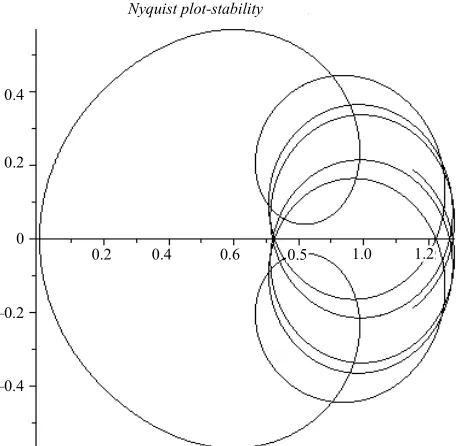
[image:4.595.308.539.85.274.2]

It’s great that all characteristic roots are in the left half plane and can stabilize the neutral system. Therefore values in (18) become the stabilizing PID parameters. Figure 1 which is plotted based on (13) shows that Ny-quist plot is in the right half plane and does not encounter the origin. According to theorem 1 the neutral system is stable. So from iteration number 2 on, the rightmost characteristic roots and consequently the stabilizing pa- rameters, are obtained. The stabilization is also proved by the closed-loop step response which is shown in Figure 2.

Moreover, as shown in Figure 3, the curve of the real parts of the rightmost characteristic roots with respect to the delay can be produced numerically by means of the proposed algorithm, which is asymptotically stable for wide range of time delays and it is shown in Figure 3 just for 



0,5000



.

4.2. Example 2

In this example we consider another neutral time-delay system with following transfer function

 









1

1 2 0.2 e s

G s

s s s 



  

Proof of stabilization

1 1.5 2 2.5

0.5 1

0.5

0

–0.58

–1

Figure 1. Proof of stabilization of Example 1 by Nyquist plot.

0 5 10 15 20

0 0.2 0.4 0.6 0.8 1

Time (sec)

Am

pl

itu

de

Step Response

Figure 2. Step response of closed-loop system at Example 1 with PID parameters at (18).

0 1000 2000 3000 4000 5000

tau

Rightmost

roots

–0.002

–0.004

–0.006

–0.008

–0.010

–0.012

–0.014

–0.016

Figure 3. The stabilizing rightmost characteristic roots for wide range of time delays.

whose closed-loop characteristic equation of system can be given by

 













3 2

1 0.2e 3 0.2e

2

d

p i

k

k k

 

  



 

     

   (19)

It can be tested that initial values have not been resulted in stability directly. By implicit differentiation, and the procedure like example 1, at iteration number 3 the rightmost characteristic roots and consequently the stabi- lizing parameters are obtained. These are obtained as

1 0.2183, 2 0.3496, 3 0.3505          and



1.0904 0.8253 0.0701



T



K ,

respectively.

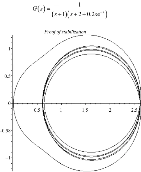
[image:4.595.306.535.319.487.2] [image:4.595.58.287.433.711.2]

resultant characteristic root (λ1 = –0.2183). The result is similar for the others and is dismissed here for brevity.

By continuing the algorithm, at the5th iteration, and at the8th iteration,



1.61 1.59 0.01T 

K



2.2 2.37 0.0012





K



_T

have been obtained, respectively. Closed-loop step re- sponse is shown in Figure 5 for PID parameters at these different iterations.

It is worthy to note that this approach does not always stop successfully in the second or third stage. Sometime it is needed to be repeated more to get the stabilizing rightmost characteristic roots and guaranteed stability. If the desired stabilizing rightmost characteristic roots have

Nyquist plot-stability

0.2 0.4 0.6 0.5

0.4

0.2

0

–0.2

–0.4

[image:5.595.58.286.253.476.2]

1.2 1.0

Figure 4. The Nyquist plot of Example 2 which does not encircle the origin.

0 5 10 15 20

0 0.2 0.4 0.6 0.8 1

Time (sec)

Am

pl

itu

de

Step Response

[image:5.595.58.292.520.707.2]

Setpoint 3rd Iteration 5th Iteration 8th Iteration

Figure 5. Step response of closed-loop system at Example 2 with PID parameters at different iterations.

not been obtained after iteration number 5, it is proposed to change the initial values of PID controller and start the algorithm from the beginning.

5. Conclusion

In the present paper, we presented an efficient and straightforward stabilizing PID controller design method for time-delay systems of neutral type which was free of mathematical complexities. Based on the proposed ap- proach, stability was guaranteed if all the characteristic roots of closed-loop system had negative real parts. For determining the rightmost characteristic roots, the meth- od was presented on the basis of Lambert W function and we managed to determine the stability directly. Delay value was chosen τ = 1 for simplicity but the algorithm could produce a plot of the real part of the rightmost root with respect to the delay as shown in the first illustrative example. Numerical examples with time delay were pre- sented for illustrating this approach. The results were satisfactory and stabilizing PID parameters were deter- mined.

REFERENCES

[1] J. P. Richard, “Time-Delay Systems: An Overview of Some Recent Advances and Open Problems,” Automatica, Vol. 39, No. 10, 2003, pp. 1667-1694.

doi:10.1016/S0005-1098(03)00167-5

[2] J. E. Normey-Rico and E. F. Camacho, “Control of Dead- Time Processes,” Springer-Verlag, London, 2007. [3] V. B. Kolmanovskii and J. P. Richard, “Stability of Some

Linear Systems with Delays,” IEEE Transactions on Automatic Control, Vol. 44, No. 5, 1999, pp. 984-989. doi:10.1109/9.763213

[4] J. K. Hale and S. M. V. Lunel, “Introduction to Func- tional Differential Equations,” Springer-Verlag, New York, 1993.

[5] L. Dugard and E. E. Verriest, “Stability and Control of Time-Delay Systems,” Springer, New York, 1998. doi:10.1007/BFb0027478

[6] S. I. Niculescu and R. Lozano, “On the Passivity of Lin- ear Delay Systems,” IEEE Transactions on Automatic Control, Vol. 46, No. 3, 2001, pp. 460-464.

doi:10.1109/9.911424

[7] K. Gu, V. L. Kharitonov and J. Chen, “Stability of Time- Delay Systems,” Birkhauser, Boston, 2003.

doi:10.1007/978-1-4612-0039-0

[8] J. R. Partingtona and C. Bonnet, “H∞and BIBO Stabili- zation of Delay Systems of Neutral Type,” Systems & Control Letters, Vol. 52, No. 3, 2004, pp. 283-288. doi:10.1016/j.sysconle.2003.09.014

[9] S. I. Niculescu, “Delay Effects on Stability: A Robust Control Approach,” Springer, New York, 2001.

1992.

[11] V. B. Kolmanovskii and V. R. Nosov, “Stability of Func- tional Differential Equations,” Academic Press, New York, 1986.

[12] J. H. Park and O. Kwon, “On New Stability Criterion for Delay-Differential Systems of Neutral Type,” Applied Mathematics and Computation, Vol. 162, No. 2, 2005, pp. 627-637. doi:10.1016/j.amc.2004.01.001

[13] V. Chellaboina, A. Kamath and W. M. Haddad, “Time- Domain Sufficient Conditions for Stability Analysis of Linear Neutral Time-Delay Systems,” Proceedings of the

2007 American Control Conference, New York, 9-13 July 2007, pp. 4917-4918.

[14] Z. H. Wang, “Numerical Stability Test of Neutral Delay Differential Equations,” Hindawi Publishing Corporation, Cairo, 2008, pp. 1-10.

[15] J. G. Ziegler and N. B. Nichols, “Optimum Settings for Automatic Controllers,” Transactions on ASME, Vol. 64, 1942, pp. 759-768.

[16] S. Yamamoto and I. Hashimoto, “Present Status and Fu- ture Needs: The View from Japanese Industry,” Chemical Process Control—CPCIV: Proceedings of 4th Interna- tional Conference on Chemical Process Control, Padre Island, 17-22 February 1991, pp. 1-28.

[17] C. Dey and R. K. Mudi, “An Improved Auto-Tuning Scheme for PID Controllers,” ISA Transactions, Vol. 48, No. 4, 2009, pp. 396-408.

doi:10.1016/j.isatra.2009.07.002

[18] B. Fang, “Computation of Stabilizing PID Gain Regions Based on the Inverse Nyquist Plot,” Journal of Process Control, Vol. 20, No. 10, 2010, pp. 1183-1187.

doi:10.1016/j.jprocont.2010.07.004

[19] N. Tan, “Computation of Stabilizing PI and PID Control- lers for Processes with Time Delay,” ISA Transactions, Vol. 44, No. 2, 2005, pp. 213-223.

doi:10.1016/S0019-0578(07)90000-2

[20] K. W. Ho, A. Datta and S. P. Bhattacharya, “Generaliza- tions of the Hermite-Biehler Theorem,” Linear Algebra and Its Applications, Vol. 302-303, 1999, pp. 135-153. doi:10.1016/S0024-3795(99)00069-5

[21] K. W. Ho, A. Datta and S. P. Bhattacharya, “PID Stabili- zation of LTI Plants with Time-Delay,” Proceedings of

42nd IEEE Conference on Decision and Control, Maui, 9-12 December 2003, pp. 4038-4043.

[22] G. J. Silva, A. Datta and S. P. Bhattacharyya, “PID Con- trollers for Time-Delay Systems,” Birkhäuser, Boston, 2005.

[23] W. Michiels, K. Engelborghs, P. Vansevenant and D. Roose, “Continuous Pole Placement Method for Delay Equations,” Automatica, Vol. 38, No. 5, 2002, pp. 747- 761. doi:10.1016/S0005-1098(01)00257-6

[24] Z. H. Wang and H. Y. Hu, “Calculation of the Rightmost Characteristic Root of Retarded Time-Delay Systems via Lambert W Function,” Journal of Sound and Vibration, Vol. 318, No. 4-5, 2008, pp. 757-767.

doi:10.1016/j.jsv.2008.04.052

[25] R. M. Corless, G. H. Gonnet, D. E. G. Hare, D. J. Jeffrey and D. E. Knuth, “On the Lambert W function,” Advances in Computational Mathematics, Vol. 5, No. 4, 1996, pp. 329-359. doi:10.1007/BF02124750