Fuzzy Neuro Model for Intelligent Credit Risk Management

Fuzzy-Neuro Model for Intelligent Credit

Risk Management

Elmer P. Dadios1, James Solis2

1_{Department of Manufacturing Engineering and Management, De La Salle University, Manila, Philippines} 2_{College of Computer Studies, De La Salle University, Manila, Philippines}

Email: elmer.dadios@dlsu.edu.ph

Received August 30, 2012; revised September 30, 2012; accepted October 8,2012

ABSTRACT

This paper presents hybrid fuzzy logic and neural network algorithm to solve credit risk management problem. Credit risk is the risk of loss due to a debtor’s non-payment of a loan or other line of credit. A method of evaluating the credit worthiness of a customer is complex and non-linear due to the diverse combinations of risk involve. To address this problem a credit scoring method is proposed in this paper using hybrid fuzzy logic-neural network (HFNN) model. The model will be implemented, tested, and validated for individual auto loans using real life bank data. The neural network is used as the learner and the fuzzy logic is used as the implementer. The neural network will fine tune the fuzzy sets, remove redundant input variables, and extract fuzzy rules. The extracted fuzzy rules are evaluated to retain the best k number of rules that will give final and intelligent decisions. The experiment results show that the performance of the proposed HFNN model is very accurate, robust, and reliable. Comparison of these results to other previous published works is also presented in this paper.

Keywords: Fuzzy Logic; Neural Networks; Fuzzy-Neuro Model; Credit Risk Management

1. Introduction

Credit scoring is a method of evaluating the credit wor- thiness of a customer. A credit scoring model is built to assist credit analysts to decide whether a new loan should or should not be granted [1,2]. The model is used as a gauge for every applicant’s profile. If a profile is equal or better than the model, the account is predicted to be “good”. Otherwise, the account is predicted to be “bad”. There have been several automated approaches presented before to solve credit scoring problem. Among them are: 1) Rule-based, 2) Statistical-based, 3) Genetic Algorithm (GA), 4) Neural Networks (NN). The rule-based (or knowledge based) approach is believed to be the easiest for a credit professional to formalize and the least expen- sive to implement [3]. It uses a set of rules derived from past credit experiences. It provides consistency to the account review process since it is an automation of the traditional risk assessment process [2]. But one major problem with rule-based scoring is the difficulty of de- termining the source of error if the system makes a series of bad decisions [3], hence, also difficult to improve. The statistical-based credit scoring method uses linear dis- criminant analysis and logistic regression. Thus, it re- quires specialized education, training and experience. Also, the traditional regression techniques cannot be fully

automated. It is labor-intensive and time consuming to design and updates the model [4]. Limited in its effect- tiveness as a long-term decision tool, the credit scoring models have to be updated and improved as trends in customer behavior changes by which the performance of the system falls below the acceptable level of prediction rate.

One of the successful techniques used to solve the credit scoring problem is the neural networks (NN) [5,6]. It is believed that NN provide an essential technology for a faster and more effective tool for credit scoring [7]. NN are capable of modeling very complex mathematical and logical relationships that are unknown to the credit ana- lyst and NN are able to model linear and non-linear rela- tionships. In terms of accuracy, in most cases, the rule- based and statistical-based credit scoring systems cor- rectly classifies at 74% [8], commercially available NN- based at 75% - 80% [8,9] and Genetic Algrithm between 72% to 74% [9].

2. The Fuzzy Logic and Neural Networks

Algorithms

and input-output relations to solve a problem. Rather, it defines complex systems with linguistic descriptions. The fuzzy logic system (FLS) contains four components: the fuzzifier, rules, inference engine and defuzzifier. The fuzzifier maps crisp input numbers into fuzzy sets. Data obtained from the outside world is converted into data understandable by the system. Rules are linguistic vari- ables expressed in IF-THEN statements. The inference engine maps fuzzy sets into fuzzy sets. It also handles situations wherein two or more rules are combined. The defuzzifier maps the fuzzy output sets into crisp outputs. The crisp output is an output that is easily understood by the outside environment.

Neural Network (NN) is an information processing paradigm that is inspired by the way biological nervous systems, such as the brain, process information [14-16]. The key element of this paradigm is the novel structure of the information processing system. It is composed of a large number of highly interconnected processing ele- ments (neurons) working in unison to solve specific problems. NN, like people, learn by example and solve problems for a specific application, such as pattern rec- ognition or data classification [16].

It has been suggested that, since all the other methods are known to possess definite advantages and disadvan- tages [2,17], the best approach is to combine the methods, taking advantage of the strengths and, thus, creating a

hybrid approach to the overall credit scoring process.

3. Hybrid Fuzzy Logic-Neural Network

(HFNN) Model for Intelligent Credit

Risk Management

The hybrid fuzzy logic neural network (HFNN) model combines the desirable properties of both neural network and fuzzy logic to form a system that supercedes the limitations of neural network and fuzzy logic algorithms. The HFNN model system learns inductively from the data using the neural network. Fuzzy rules are extracted from the trained neural network and with the extracted rules, previously unseen data can be discriminated whe- ther “good” or “bad” accounts.

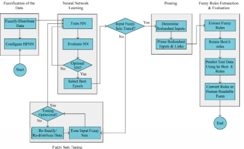
The HFNN model developed in this paper undergoes two stages, namely: learning (or training) and implemen- tation (or testing). Figure 1 shows the learning stage of the HFNN model. The different phases that took placed in the learning stage are: Fuzzification of the Data, Neu- ral Network Learning, Fuzzy Sets Tuning, Pruning Input Variables, and Fuzzy Rule Extraction & Evaluation.

3.1. Fuzzification of Data

The fuzzification of data is conducted and configured manually. All fuzzy sets are initialized before the training data are inputted into the neural net. The input variables

are partitioned by overlapping fuzzy sets and the mem- bership functions are initialized based on the recommen- dation of a loan evaluation expert [18]. Note that the specification of membership function is subjective and may vary from different experts. However, membership functions cannot be assigned arbitrarily. The number of membership functions is chosen such that the resulting fuzzy rules will be easily readable and accurate enough to classify data. Figure 2 shows sample typical fuzzy sets for an input variable Total Income.

The fuzzification and distribution of data are auto- mated processes. Through the fuzzy sets, the crisp input from 1000 samples is fuzzified one at a time and serves as a fuzzy input to the NN [19]. To fuzzify a crisp input, the degree of membership of the crisp input in each of the affected fuzzy members is computed. The fuzzy member that gets the bigger degree of member gets the value 1, the rest of members get the value 0. In case, the degree of member is the same for 2 adjacent fuzzy members, the leftmost member gets the value 1. The rightmost member gets the value 0. For example, as shown in Figure 2, when Income = P45,000 and based in the membership functions shown, the degree of mem- bership of P45,000 is 7/8 in Low and 1/8 in Medium.

Hence, μ(45,000) = max(7/8, 1/8) = 7/8

So, μ(45,000) is Low, which means that the Total In- come is Low. The data then are distributed after fuzzify- ing the entire 1000 samples. The first 630 samples be- comes the training set, the next 70 samples becomes the evaluating set, and the last 300 samples becomes the testing set.

3.2. Neural Network Learning for HFNN Model

In this research, the neural network (NN) learns purely

Figure 2. Sample fuzzy sets for an input variable total in-come.

from the training data presented to the model. The NN is initialized with input neurons equal to the number of fuzzy input members. This means that for every fuzzy input member there should be a corresponding neuron in the NN. Hence, for the input variable Total Income shown in Figure 2, there must be also 4 input neurons in the NN shown in Figure 3. The output layer has two neurons one for good and the other one for bad [19,20]. The number of hidden neurons is 2/3 of the sum of the total number of input neurons plus the total number of the output neurons [21].

The neural network is trained using backpropagation method to map the fuzzified inputs to the desired output [14]. The optimum accuracy is achieved when the classi- fication error is minimized for the training data and at the same time giving the best accuracy performance for the validation data. When the neural network attained opti- mum classification accuracy, fuzzy rules are extracted from the NN. The extracted rules are used by the fuzzy system during the implementation for the classification of the previously unseen samples.

3.3. Fuzzy Input Set Tuning

The tuning process of fuzzy input sets is conducted automatically [19]. Only inputs that are continuous vari- ables are tuned. Adjustment on the boundaries of the fuzzy members of a given fuzzy set follows specific re- straints. In this paper, the following restrictions are ada- pted:

1) The fuzzy sets are kept overlapped with the adjacent fuzzy sets, as shown in Figure 2.

2) When updating the parameters, the parameters a, b, and c should remain valid; that is l ≤a ≤b ≤c ≤u must always hold, where [l, u] is the domain of the corre- sponding variable.

3) When updating the position parameters of the cur- rent fuzzy member, the parameters of current member should not become smaller than the corresponding pa- rameters of the left neighbor or larger than the corre- sponding parameters of the right neighbor.

4) The parameter a of the leftmost member and the parameter c of the rightmost member remain fixed.

5) The parameter b of the current fuzzy member being updated should not become greater than the parameter c of the right member or smaller than the parameter c of the left member.

Figure 3. Architecture of fuzzy input to the NN during learning stage.

racy for the newly tuned fuzzy input sets [18,19].

3.4. Pruning the Input Variables or Fuzzy Sets

Pruning or removal of redundant input variables or fuzzy sets will improve the readability of a fuzzy rule base ex- tracted during the learning stage. Removal of the redun- dant input fuzzy sets will simplify the model. Pruning techniques are adapted from NN wherein, tests are made for its parameters. i.e. either weights or neurons to de- termine how the error would change if the parameter is removed [20]. In this paper, fuzzy sets that represent va- rious input variables in all possible combinations are re- moved and the network classification performance is evaluated.

The process in determining redundant variables is con- ducted by systematically enabling or disabling the inputs. When an input is enabled, its contribution is accepted into the NN. But when an input is disabled, its value is blocked in the NN. It is as if the input does not exist. With all the possible combination of enabled and dis-abled inputs, the prediction accuracy of each combina-tion is recorded.

In this study, the 16 input variables shown in Table 1 is presented in binary and equivalent to 216_{− 1 or 65,535}

combinations. For a given sample, the HFNN model may take in the values of 2 input variables, e.g., Age and To- tal Income, and ignoring the values of the remaining 14 input variables. This is one unique combination of the inputs. The ignored values of input variables are changed to zero before being inputted to the hybrid network. This is to neutralize the effect of the input variables that are not included in that particular combination. The 65,535 unique combinations will be ranked according to their accuracy performance. Among the combinations with the

same accuracy performance, say 100%, the combination with the least number of fuzzy inputs and maximum num- ber of rules is the most desirable combination.

3.5. Fuzzy Rule Extraction and Evaluation

From the pruned system, all possible fuzzy rules are ex- tracted. Figure 4 shows how to extract fuzzy rules in the HFNN model. The combination pattern 0 3 0 2 is the exact representation of the fuzzy inputs combination both enabled and disabled. The zero value represents disabled input. With the output of G for Good, 0 3 0 2 G is one fuzzy rule. Every possible combination of the fuzzy in- puts is considered a rule. This rule is being evaluated by NN whether the combination results is “good” or “bad”. Note that rules are derived from unique combinations of the enabled fuzzy inputs. There are no two rules that have exactly the same combination of the enabled fuzzy inputs. Hence, there are no conflicting rules that results from these combinations.

Table 1. Snapshot of a single record in the sample data.

Input/Variable Name Variable Type *_{Original Record Converted Record No. of Fuzzy members Fuzzified Record}

1) Age *_{Cont. 39 39 4 0100}

2) No. of Dependents Cont. 2 2 4 1000

3) Length of Service Cont. 10 10 4 1000

4) Total Income Cont. 225,000 225,000 4 0001

5) Term of Loan Cont. 18 18 5 01000

6) GMI Ratio Cont. 18.04 18.04 4 0100

7) Equity Ratio Cont. 55.56 55.56 4 0001

8) Employment Type *_{Categ Self-employed 2 2 01}

9) Civil Status Categ Married 1 6 100000

10) Gender Categ. Male 1 2 10

11) Type of Residence Categ. Owned 1 4 1000

12) Type of Neighborhood Categ. Average 2 5 01000

13) Credit Experience Categ. Up-to-date 1 14 10000000000000

14) Nature of Business Categ. Comm’ty/social service 6 11 00000100000

15) Court Case Categ. w/o court case 1 2 10

16) Landline Availability Categ. w/home phone 1 4 1000

*_{This is the first record in the sample data. Cont.—Continuous. Categ.—Categorical.}

Figure 4. Extracting rules from the HFNN model.

define the credit scoring model. Figure 5 shows the sam- ple diagram of the process for getting the best k rules.

3.6. Fuzzy Logic Implementation Stage of HFNN Model

The optimized fuzzy sets achieved during the learning stage are used in the implementation stage. The test sam- ples are first fuzzified through these optimized fuzzy sets before these input are inferred with the fuzzy rule base. Once the rules are evaluated and compiled, each fuzzi-

fied input is compared with the compiled rules and are classified, as shown in Figure 6. If corresponding rule is not found, the input is classified as unclassified. Other- wise, input is classified either as correctly classified or misclassified.

A sample miniature compilation of the fuzzy rules learned and evaluated from the learning data are as enu- merated below:

Combination Pattern Output xTime u

0 1 0 1 B 0 0 2 0 1 B 2 0 3 0 1 B 1 0 4 0 1 G 4 0 1 0 2 B 1 0 2 0 2 G 8 0 3 0 2 G 2 0 4 0 2 G 0

sed

8 Rules Training Samples

0 2 0 1 B 0 2 0 2 G 0 3 0 1 G 0 4 0 1 G .

. .

0 2 0 2 G 0 3 0 2 G .

. .

0 1 0 2 B 0 3 0 1 B

6 Rules

Combination Pattern Output xTime

0 2 0 2 G 8 0 4 0 1 G 4 0 2 0 1 B 2 0 3 0 2 G 2 0 3 0 1 B 1 0 1 0 2 B 1

used

Combination Pattern Output xTime used

0 2 0 2 G 8 0 4 0 1 G 4 0 2 0 1 B 2 0 3 0 2 G 2

4 Best Rules

Figure 5. Illustration of retaining the best k rules.

Figure 6. Architecture of the fuzzy logic implementation stage of the HFNN model.

2) IF Total Income is High AND Civil Status is Mar- ried AND Age is Middle THEN Account is GOOD.

3) IF Total Income is High AND Civil Status is Single AND Age is Old THEN Account is BAD.

The Classification of the data is the end result of the process. A sample classification of the systems is shown below:

1) IF Total Income is High AND Civil Status is Mar- ried AND Age is Middle.

A fuzzified account that is actually BAD but is in- ferred by the fuzzy rule base as GOOD is a misclassifica- tion.

2) IF Total Income is Low AND Civil Status is Single AND Age is Young.

This account is actually GOOD and classified as GOOD is correctly classified.

3) IF Total Income is Low AND Civil Status is Mar- ried AND Age is Young

If this account cannot be found in the fuzzy rule base then it is unclassified.

Table 1 presents sample data record, from its original form to its fuzzified form. Just refer to section 4.1 for more details.

4. Experiment Results

4.1. Description of Experiment Data

In this research a total of one thousand records from the bank were selected uniformly to be used for experiments. There are 630 “good” and 370 “bad” of the thousand accounts selected. The data contains 16 variables, shown in Table 1. These 16 variables were used by statistical tool of the bank in assisting the human credit evaluators in reviewing the loan applications. Also, the same input variables were considered in earlier credit scoring sys- tems developed and published as described in section 1.

because only 14 out of the 1000 accounts selected have “With” court case value and 986 accounts have “With- out” court case value.

Epoch 700 600 500 400 300 200 100 0 -100 C la s sif ica ti o n , % 102 100 98 96 94 92 90 88 4.2. Traditional Neural Network (MLP)

Experiments Results

In this research, experiments using traditional NN (Multi Layer Perceptron) is conducted and compared to the pro- posed HFNN model developed. Figures 7 and 8 shows the results of the NN training and samples classification performance. Figure 7 presented a typical behavior of a neural network that is being trained. It just continuously learned and cross-validation was used to determine when the training stopped. When compared to the performance of the proposed HFNN model shown in Figure 9, the traditional NN performance does not indicate any spike because there was no fuzzy input tuning process that hap- pened.

EV samples

TE samples

TR samples

It can be observe from Figure 8 that the patterns of training (TR), evaluation (EV), and testing (TE) samples are similar. When one group of samples, say TR, are de- creasing in classification accuracy, the other groups are also decreasing. Moreover, Figure 8 shows that as clas- sification rate for the TR samples is still increasing, the

Epoch 400000 200000 0 -200000 A v e . S q rd . E rro r (in E -0 2 ) 50 40 30 20 10 0 800000 600000

Figure 7. Neural network training performance.

y Epoch 600000 400000 200000 0 -200000 C lassi fi ca ti on, % 100 90 80 70 60 800000

T E samples

EV samples

T R samples

Figure 8. Neural network classification accuracy compari-son.

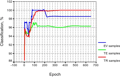
Figure 9. HFNN model classification performances.

classification rates for EV and TE samples are already declining. This is an indication that the network is getting over-fitted for TR samples. Hence, the training is stopped. The final classification accuracy on this experiment is 94.67%. However, it is important to note that the training of the traditional MLP to get optimum accuracy took longer time compared to the proposed HFNN Model. It recorded and average of 48 hours to train the MLP for each set using Pentium 4 - 2.8 GHz Single Core Proces- sor with 512 Mb RAM.

4.3. The Proposed HFNN Model Experiments Results

Figure 9 shows the performance of the proposed HFNN model developed in this research. It can be seen from the graph that each group of the samples behave similarly as the system is being trained. The classification accuracies of Training (TR), Evaluation (EV), and Testing (TE) samples were already dropping after the 25th epoch. However, when the tuning process for input fuzzy set is activated all classification accuracies started to improve particularly the EV samples, which reached 100% accu- racy from 77th epoch to 197th epoch. The classification accuracy of the system for the training samples (TR) started to slow down at 117th epoch. However, at 347th epoch the system achieved 100% classification accuracy. The evaluation samples (EV) had reached 100% classify- cation accuracy at 77th epoch. However it was over-fit- ted after the 197th epoch. Hence, a drop in the classifica-tion accuracy for EV begun until it settled at 98% classi-fication accuracy at 247th epoch.

The test samples, TE, on the other hand, were classi- fied by the system as having patterns much similar with EV. But the graph in Figure 9 shows that the TE samples have more patterns that are diverse than that of EV sam- ples. That is why, TE classification rate dropped earlier and lower than EV. TE classification rate reached 96%. The tuning of the fuzzy sets served its purpose—the classification performance of the HFNN Model had im- proved so much. As can be seen in Figure 9, all three graphs were falling continuously until at their lowest at 47th epoch.

4.4. Performance Comparison of the Proposed HFNN Model against Traditional Neural Network (MLP)

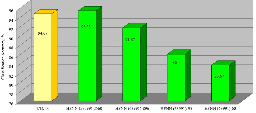
Figure 10 shows the behavior of the proposed HFNN model against the traditional NN developed in this re- search. Both of these two models showed superior per- formance against the previous published works men- tioned in Section 1. It can be seen from this figure that the highest TE classification accuracy equal to 95.33% ob- tained by the proposed HFNN model using 2560 rules. The neural network classification accuracy is lower than this at 94.67%.

Furthermore, it can be observed that using HFNN mo- del with 95 rules resulted to 86% classification accuracy. It even dropped to 83.67% when using 60 rules. This is a trade-off of the system developed which the human ex-perts have to decide. It should be noted that minimizing the number of rules and input variables will make easy and simple for the human credit evaluators to read and decide. The simplification of the rules may result the ex- pense of the classification accuracy. However, in this

proposed HFNN model, the 83.67% classification accu-racy using 60 rules is still way above acceptable than that of classical method reported in Section 1 mentioned ear- lier in this paper.

The training time of the proposed HFNN model to get optimum accuracy performance took only 3 hours com- pared to 48 hours of the traditional Multilayer Perceptron (MLP) Neural Network. The fuzzification increased the granularity of the continuous input values. The complex- ity of the various patterns found in the samples was re- duced, and so with the training time as a consequence.

5. Discussion and Analysis of Results

In this research, the developed HFNN model tuning process improved the classification accuracy signifi- cantly. Without tuning process, the classification accura- cies of the 3 sets; TR, EV, and TE could have been peg to 94%. But employing the tuning process, TR samples had reached and set at 100%, EV samples at 98.57% and TE samples at 96%. This can be seen in Figure 9.

The original HFNN model with complete 16 input variables got a classification accuracy of 98.57% only when tested with the evaluating samples (EV). When the redundant input variables were removed, the perform- ance improved to 100%. The improvement signified that some input variables or their particular combinations contributed to noise. Hence, the removal of the redundant input variables not only improved the readability of the rules but it also improved the accuracy performance of the HFNN model developed.

The improvement of the rule base can be defined in terms of performance (i.e. reduction of error) and in terms of complexity or simplicity (i.e. number of variables or

95.33 94.67

91.67

86

83.67

76 78 80 82 84 86 88 90 92 94 96

NN-16 HFNN (57599)-2560 HFNN (63991)-896 HFNN (63991)-95 HFNN (63991)-60

Clas

si

fi

ca

tion A

cc

ur

ac

y,

%

parameters). There is a trade-off between performance and simplicity. To obtain high accuracy, a large number of free parameters are needed, which again resulted in a very complex and thus less comprehensible or readable model. However, often the performance of a model can actually increase with the reduction of the number of parameters because the generalization capabilities of the model may increase. If the model has too many parame- ters, it tends to over-fit the training samples, TR, and displays poor generalization on test samples, TE.

The removal of 12 input variables found to be redun- dant resulted to 896 extracted rules only. Eliminating the 836 noise rules, the ones with single or no “hits” in the training set, further simplified the readability of the set of rules down to 60 rules. These 60 rules define the credit scoring model with a classification performance of 83.67% when tested with the test set, way above the in- dustry standard of 74% classification performance. Fi- nally, The HFNN model developed in this research trains faster than the traditional NN by 16 times and has better classification accuracy of 95.33% compared to 94.67% of traditional NN.

6. Conclusions and Recommendations

The HFNN model developed in this research to solve credit risk management problem is capable of self- learning similar to the traditional neural network. Subse- quently, once trained, it is capable of discriminating the “good” and the “bad” accounts with better accuracy compared to the traditional NN. Unlike the neural net- work’s “black box” configuration, which is an undesir- able feature for credit evaluation, the HFNN model is capable of generating the rules behind the discrimination of each account subjected to it. The system behaves much like a traditional fuzzy logic system in this aspect. However, the HFNN model is better than the traditional fuzzy logic system because of its learning capability. The fuzzy logic system does not have this capability.

Although, this research was done for auto loan, the Hybrid Fuzzy-Neuro Network is easily transferable to similar loan products like mortgage loan, salary loan, and even for credit card grants. These types of loans are the same because they have similar input and output vari- ables required.

In this research, the extracted rules were just listed in the order of their importance, i.e. the most relevant rules were listed first in the list. For future works, it is worth to investigate some of these rules that can be fussed to- gether to further simplify the list of rules. The output of the developed HFNN model is limited to 2 possible val- ues; either good or bad. By providing the data with more than 2 outputs, say 2 additional outputs, namely: margin- ally good and marginally bad. Marginal accounts can be

taken for a closer look before a decision is granted. This can be considered for future study.

REFERENCES

[1] M. Bonilla, I. Olmeda and R. Puertas-An, “Application of Genetic Algorithms in Credit Scoring,” WASL Journal, 2000.

[2] L. P. Wallis, “Credit Scoring,” Business Credit Magazine, March, 2001.

[3] A. Fensterstock, “Credit Scoring Basics,” Business Credit, March, 2003.

[4] A. Jost, “Neural Networks,” Credit World,Vol. 81, No. 4, 1993, p. 26.

[5] A. Fensterstock, “The Application of Neural Networks to Credit Scoring,” Business Credit, March, 2001.

[6] G. Vasconcelos, P. Adeodato and D. S. M. P. Monterio, “A Neural Network Based Solution for the Credit Risk Assessment Problem,” Proceedings of the IV Brazilian Conference on Neural Networks, Washington, 20-22July 1999, pp. 269-274.

[7] S. A. DeLurgio and F. Hays, “Understanding the Finan-cial Interests in Neural Networks,” WASL Journal,2001.

[8] BrainMaker, “Credit Scoring with Brainmaker Neural Network Software,” 2003.

http://www.calsi.com/CreditScoring.html

[9] J. Whitehouse, “Human Capabilities + Computer Auto-mation = Knowledge,” IT Briefing, Pacific Lutheran Uni-versity, Parkland, 2000.

[10] E. P. Dadios and D. J. Willaims, “A Fuzzy-Genetic Con-troller for the Flexible Pole-Cart Balancing Problem,”

Proceedings of 1996 IEEE International Conference on Evolutionary Computation,Nagoya, 20-22 May 1996, pp. 223-228.

[11] L. A. Zadeh, “A Theory of Approximate Reasoning,” In:

Machine Intelligence, John Wiley & Sons, New York, 1979, pp. 149-194.

[12] I. Iancu, “A Mamdani Type Fuzzy Logic Controller,” In: E. P. Dadios, Ed., Fuzzy Logic: Controls, Concepts,

Theories and Applications, InTech Croatia, Rijeka, 2012, pp. 55-54.

[13] A. Achs, “From Fuzzy Datalog to Multivalued Knowl-edge-Base,” In: E. P. Dadios, Ed., Fuzzy Logic: Algo-rithms, Techniques and Implementations,InTech Croatia, Rijeka, 2012, pp. 25-54.

[14] E. P. Dadios, K. Hirota, M. Catigum, A. Gutierrez, D. Rodrigo, C, San Juan and J. Tan, “Neural Network Vision Guided Mobile Robot for Driving Range Golf Ball Re-triever,” Journal of Advanced Computational Intelligence and Intelligent Informatics,Vol. 10, No. 4, 2006, pp. 181- 185.

[15] R. Gustilo and E. P. Dadios, “Optimal Control of Aqua-culture Prawn Water Quality Index Using Artificial Neu-ral Networks,” Proceedings of the 5th IEEE International Conference on Cybernetics and Intelligent Systems and the 5th IEEE International Conference on Robotics,

Septem-ber 2011, pp. 266-271.

[16] S. Hilado and E. P. Dadios, “Face Detection Using Neural Networks with Skin Segmentation,” Proceedings of the

5th IEEE International Conference on Cybernetics and Intelligent Systems and the 5th IEEE International Con-ference on Robotics, Automation and Mechatronics, Qingdao, 17-19 September 2011, pp. 261-265.

[17] N. Marcos, “Belief-Evidence Fusion through Successive Rule Refinement in a Hybrid Intelligent System”, Ph.D. Thesis,De La Salle University, Manila, 2002.

[18] D. Nauck, “Combining Neural Networks and Fuzzy

Con-trollers,” FLAI, Linz, 28 June-2 July 1993.

[19] D. Nauck, “Data Analysis with Neuro-Fuzzy Methods,” Habilitation Thesis, University of Magdeburg, Magde-burg, 2000.

[20] S. Haykin, “Neural Networks: A Comprehensive Founda-tion,” Prentice Hall, Upper Saddle River, 1999.