Experimental study and modelling of average void fraction
of gas-liquid two-phase flow in a helically coiled
rectangular channel
XIA, Guodong, CAI, Bo, CHENG, Lixin, WANG, Zhipeng and JIA, Yuting Available from Sheffield Hallam University Research Archive (SHURA) at: http://shura.shu.ac.uk/18593/
This document is the author deposited version. You are advised to consult the publisher's version if you wish to cite from it.
Published version
XIA, Guodong, CAI, Bo, CHENG, Lixin, WANG, Zhipeng and JIA, Yuting (2018). Experimental study and modelling of average void fraction of gas-liquid two-phase flow in a helically coiled rectangular channel. Experimental Thermal and Fluid Science, 94, 9-22.
Copyright and re-use policy
See http://shura.shu.ac.uk/information.html
Sheffield Hallam University Research Archive
1
Experimental study and modelling of average void fraction of gas-liquid two-phase
flow in a helically coiled rectangular channel
Guodong Xiaa* Bo Caia Lixin Chenga,b* Zhipeng Wanga Yuting Jiaa
a
College of Environmental and Energy Engineering, Beijing University of Technology,
Beijing, 100124, China
b
Department of Engineering and Mathematics, Faculty of Arts, Computing, Engineering
and Sciences, Sheffield Hallam University, UK
*Corresponding author: Tel.:+86 10 67391985-8301; fax: +86 10 67391983. *Email
address: [email protected]; [email protected]
Abstract
Void fraction is an important parameter in designing and simulating the relevant
gas-liquid two-phase flow equipment and systems. Although numerous experimental
research and modelling of void fraction in straight circular channels have been conducted
over the past decades, the experimental data and prediction methods for the average void
fraction in helically coiled channels are limited and needed. Especially, there is no such
information in helically coiled channels with rectangular cross section. Therefore, it is
essential to advance the relevant knowledge through experiments and to develop the
corresponding prediction methods in helically coiled rectangular channels. This paper
2
fraction in a horizontal helically coiled rectangular channel. First, experiments were
conducted with air-water two-phase flow in the horizontal helically coiled rectangular
channel at a wide range of test conditions: the liquid superficial velocity ranges from 0.11
to 2 m/s and the gas superficial velocity ranges from 0.18 to 16 m/s. The average void
fractions were measured with a quick-closing valve (QCV) method. The measured void
fraction ranges from 0.012 to 0.927 which cover four flow regimes including unsteady
pulsating, bubbly, intermittent and annular flow observed with a high speed camera. Second,
comparisons of the entire measured average void fraction data to 32 void fraction models
and correlations were made. It shows a low accuracy of these models and correlations in
predicting the experimental data for the void fraction smaller than 0.5 while the drift flux
model of Dix [Woldesemayat and Ghajar, Int. J. Multiphase Flow. 33 (2007) 347-370.]
predicts 98.3% of the entire experimental data within ±10% for the void fraction larger than
0.5. Therefore, the Dix model is recommended for the void fraction larger than 0.5.
Furthermore, the observed flow regimes in the coiled channels were compared to two
mechanistic flow regime maps developed for horizontal straight circular tubes. The flow
regime maps do not capture all flow regimes in the present study. Finally, the effects of the
limiting affecting parameters on the void fraction models are analyzed according to the
physical phenomena and mechanisms. Incorporating the main affecting parameters, new
void fraction models have been proposed for the void fractions in the ranges of 0 < α ≤ 0.2
and 0.2 < α ≤ 0.5 respectively according to the slip flow model. Both models predict the
experimental data reasonably well. Overall, the new proposed models and the
3
Keywords: air-water two-phase flow; helically coiled rectangular channel; flow regime;
void fraction; experiment; model
1. Introduction
Gas-liquid two-phase flow in helically coiled channels is frequently encountered in
various industrial units such as various heat exchangers, power generations, nuclear
reactors, oil-gas process systems, gas-liquid mixing units and so on [1, 2]. Understanding
the channel average void fraction of two-phase flow is significant and necessary for
modelling the flow regimes and their transitions, the two-phase pressure drop and phase
change heat transfer in various gas-liquid two-phase flow systems [3-5]. Accurate
knowledge of the average void fractions of gas-liquid two-phase flow is significant in
modelling the numerical computation and beneficial to the design and application for
various industrial processes.
A number of researchers have conducted experimental investigations on the void
fraction in straight circular tubes under various conditions such as flow boiling,
condensation and adiabatic two-phase flow. Srisomba and Mahian [6] conducted the
experiments to measure the void fraction of R-134a in a horizontal circular tube using a
quick-closing valve (QCV) method and optical observation techniques. Based on their
measured void fraction, they have proposed new correlations for predicting the void
4
angles on the void fraction, which closely related with flow regimes during condensation
with R134a inside smooth tubes. Jagan and Satheesh [8] investigated the flow regimes and
the void fraction of air-water two-phase flow in a circular tube at different inclination
angles ranging from 0° to 90°. The void fractions were measured using the QCV method in
their study. Milkie [9] investigated the flow regimes and void fractions for condensation of
propane flowing through horizontal tubes with a diameter of 7 mm and 15 mm. Detailed
analyses of the video frames were used to develop a new multi-regime void fraction model
based on the drift flux model. The model provides improved agreement with the
experimental results when compared to correlations in the literature. Lockanathan and
Hibiki [10] presented a comprehensive review and analysis of the flow regime, void
fraction and pressured drop for downward two-phase flow and pointed out the future
research needs in their review. Just to name a few studies of void fraction in straight tubes
here. Furthermore, the available prediction models and correlations for the void fraction in
the two-phase flow have been extensively developed for straight circular channels [11].
However, studies of the void fraction of gas-liquid two-phase flow in helically coiled
channels are very limited. Due to the centrifugal acceleration effect which generating the
secondary flow in the main two-phase flow, the flow structure and the relative motion
between phases in a helically coiled channel are much more complicated than those in a
straight tube. In particular, studies of the void fraction and flow structure for gas-liquid
two-phase flow in a helically coiled rectangular channel are very limited in the literature so
far. Recently, Liu et al. [15] investigated the characteristics of air-water two-phase flow in a
5
structure using a high speed video system. They indicated that the presence of the
secondary flow leading to a complex asymmetry phase distribution for two-phase flow in
the helically coiled rectangular channels. They illustrated the flow pattern evolutions in
different position of the helically coiled rectangular channels. However, their study does
not concern the void fraction in the helically coiled rectangular channels, which is
important in understanding the fundamentals of gas-liquid two-phase flow and worth being
investigated in such a coiled channel with non-circular shape.
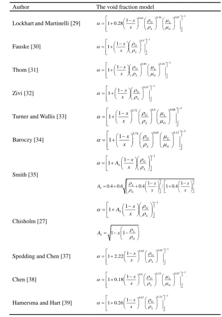
Furthermore, there are many void fraction correlations/models available in the
literature. Based on the major three typical models, i.e. homogeneous model, slip flow
model and drift flux model. Many models and correlations for predicting the void fraction
were developed based on these models. Woldesemayat and Ghajar [11] investigated the
predictive performance of 68 void fraction models and correlations for straight tube with
different orientations. Xue [12] did a comparative work to evaluate the accuracy of 39
models and correlations for calculating void fraction in downward two-phase flow system.
Jagan and Satheesh [8] measured void fraction in straight tubes under different inclined
angles and compared with five existing correlations. Mandal and Das [13] and Biswas and
Das [14] investigated the two-phase pressure drop and the liquid holdup with three varying
gas-non-Newtonian two-phase flow for both horizontal and vertical helical coils with
circular cross section. They presented the void fraction correlations for helically coiled
channel by dimensionless analysis. Furthermore, Xia and Liu [15-17, 36] investigated the
effect of liquid holdup on the phase distribution and pressure drop of two-phase flow in
6
nearly all the available void fraction models and correlations of air-water two-phase flow
were developed for straight circular tubes. It is unclear if these correlations are applicable
to helically coiled rectangular channels. Furthermore, flow regimes are intrinsically related
to the corresponding void fractions. It is essential to predict the flow regimes properly using
the relevant flow regime map when developing the relevant prediction methods for the void
fractions. Several mechanistic flow regime models and maps have been developed for flow
regime pattern prediction, i.e. the mechanistic maps and models of Taitel and Dukler [53],
Taitel [54] and Zhang et al. [55-57]. These maps and models are generally applicable to
straight circular channels. For the flow regimes in the coiled rectangular channels in the
present study, it is essential to evaluate the mechanistic flow regime maps and models with
the experimental data in such channels. Due to the secondary flow generated in the coiled
channels, possible different flow regimes may occur in such channels.
To the authors' knowledge based on the literature review, the experimental data and
prediction methods for the average void fraction of two-phase flow in helically coiled
channels are limited. Especially, there is no such information in helically coiled channels
with rectangular cross section so far. Therefore, it is essential to conduct experiments to
measure the average void fractions of gas-liquid two-phase flow in the helically coiled
rectangular channels and to develop new models for predicting the void fraction if the
existing models do not work, which are the objectives of the present study.
In this study, the experimental results of the average void fractions corresponding to
the flow regimes observed with the high speed video camera are presented at first. Then, 32
7
measured void fraction data. Furthermore, the mechanistic flow regime maps of Taitel and
Dukler [53] and Zhang et al. [55, 56] have been evaluated with the observed flow regimes
in the coiled channel. Finally, new models have been proposed for the helically coiled
rectangular channel according to the void fraction ranges and the relevant physical
phenomena and mechanisms.
2. Experimental setup, test section and measurement system
An experimental system was designed and built to measure the average void fractions
and to observe the flow regimes of air-water two-phase flow in the horizontal helically
coiled rectangular channel simultaneously by the QCV method and the flow visualization
method with the high speed video camera respectively. The experimental setup, test section
and measurement system are described here.
2.1. Experimental setup
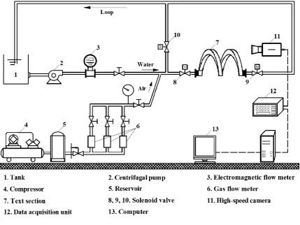
Figure 1 shows the schematic diagram of the experimental setup for air-water
two-phase flow for the measurement of the void fraction in the test channel. It consists of
air and water supply system including pipes and valves (8), (9) and (10), the test section (7),
measurement system and data acquisition system including a data acquisition unit (12) and
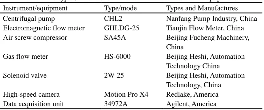
a computer (13). The types, modes and manufactures of the instrument and equipment used
in the experiments are shown in Table 2. Water is supplied by a centrifugal pump (2) from a
8
then stored in the air reservoir (5) at a pressure of 0.8 Mpa. The reservoir (5) is used to
maintain stable air flow in the experimental system. The flow rate of air is measured by
three gas flow-meters (6) with an accuracy of ±1.5%. The flow rate of water is measured by
an electromagnetic flow-meter (3) with an accuracy of ±0.5%. The water flow rate can be
adjusted with an adjustable valve in the water supply line to a desired superficial liquid
velocity in the experiments. The three flow meters are used to achieve the wide range test
range of superficial velocities from low to high values. Three values after the gas flow
meters are used to adjust the air flow rate to a desired gas superficial velocity in the
experiments. Air and water are well mixed in a Y-connection mixer before the test section,
which has a straight branch for liquid flow and air injected in the side-way. Then, the
air-water two-phase mixtures flow into the test section (7) which is the horizontal helically
coiled rectangular channel, where the QCV method including two solenoid valves (8) and
(9) is used to measure the average void fraction and the Motion Pro X4 high speed video
camera (11) is used to observe the flow regimes simultaneously. The pipe between the
Y-mixer and the test section is long enough to ensure that the gas-liquid two-phase flow is
stable in the experiments. Finally, the two-phase fluids flow back to the water tank which is
open to the atmosphere. The water returns to the water tank (1) and the air vents into the
atmosphere.
2.2. Test section
The test section is a transparent helically coiled rectangular channel which is made of
9
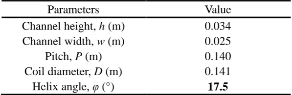
coiled rectangular channel and its geometry dimensions. Table 1 lists the geometry
dimensions of the test section corresponding to Figure 3. The coil diameter D of the
helically coiled rectangular channel is 141 mm and its pitch P is 140 mm. The helix angle
of the test section is 17.5º. The dimensions of its rectangular cross-section is: w × h = 25
mm (width) × 34 mm (height). For the non-circular channel, equivalent diameters rather
than hydraulic diameters is used in gas-liquid two-phase flow as suggested by Cheng et al.
[18-20] and Moreno Quibén et al. [21, 22]. The equivalent diameter dE of the rectangular
channel is defined as
R
4 4
E
A wh
d
(1)
where AR is the cross-section area of the rectangular coiled channel. It should be pointed
out that using the equivalent diameter gives the same mass velocity as in the non-circular
channel and thus correctly reflects the mean liquid and vapor velocities, something using
hydraulic diameter in a two-phase flow does not [18-22].
2.3. Measurement system
The measurement system consists of flow meters for the liquid and gas flow rates,
measurements of the average void fractions with the QCV method and observing the
corresponding flow regimes with the high speed video camera simultaneously. The
sampling frequency of the high speed video camera is 1000 frames per second. The
10
by the Agilent 34972A data acquisition system (DAS) and a computer. The measured data
were stored in the computer for future data reduction and analysis.
Figure 4 shows the principle of measuring the void fraction with the QCV method.
Two normally opened solenoid valves (8) and (9) are mounted at the inlet and the outlet of
the test section respectively. One normally closed solenoid valve (10) is mounted in the
bypass line. The three solenoid valves can function simultaneously while the same power
supply is connected to the three actuators of the solenoid valves.
The channel average void fraction of gas-liquid two-phase flow in the tested helically
coiled rectangular channel with the QCV method can be calculated as follows:
1
1 1
n
i i
M
n M
(2)where M is the mass of water filled in the test section, Mi is the water mass of two-phase
flow remained in the test section, n is the number of measurements at a given flow
condition. The mass of water remaining in the channel is measured by using an electronic
balance with high accuracy. The measurements are repeated at least five times for each test
run and the average result of all the measurements for the test run is used as the measured
average void fraction.
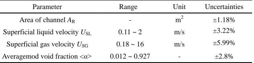
2.4. Experimental conditions and measurement uncertainty analysis
11
The density of water and air are 998.2 and 1.205 kg/m3 respectively and the dynamic
viscosity of water and air are 1.004×10⁻³ and 1.81 ×10⁻⁵ m2/s respectively. Wide ranges of
liquid and gas superficial velocities were used to cover a wide range void fractions in
various flow regimes in the test section. Table 3 lists the experimental conditions. The
liquid superficial velocity varies from 0.11 to 2 m/s and the gas superficial velocity varies
from 0.18 to 16 m/s. With the test conditions, the channel average void fraction is in the
range from 0.012 to 0.927.
The measurement uncertainties were analyzed with the methods of Taylor [23] in this
study. Table 3 shows the uncertainties of measurement parameters. The processing
precision of channel width and height is less than 0.5 mm. the uncertainty of channel
cross-section area is estimated to be about ±1.18%. The uncertainty of the liquid superficial
velocity is ± 3.22%. The uncertainty of the gas superficial velocity is ± 5.99%. The
uncertainty of channel average void fraction is ± 2.8%.
3. Experimental results and analysis
The average void fraction of gas-liquid two-phase flow were measured in the
horizontal helically coiled rectangular channel by using the QCV method in wide range of
gas and liquid superficial velocities: 0.18 < USG < 16 m/sand0.1 < USL < 2 m/s. The
corresponding flow regimes were simultaneously observed with the high speed video
camera. Four main flow regimes were observed in the test helically coiled rectangular
12 annular flow.
Figure 5 shows the measured average void fractions at the liquid superficial velocities
of 0.098, 0.196 and 0.294 m/s and a photograph of the observed unsteady pulsating flow
regime which occurs at a medium range of the void fraction from about 0.3 to 0.75. Figure
6 shows the measured average void fractions at the liquid superficial velocities of 0.882,
0.98, 1.378 and 1.905 m/s and a photograph of the observed the bubbly flow regime which
occurs at a low range of the void fraction from about 0.008 to 0.18. Figure 7 shows the
measured average void fractions at the liquid superficial velocities of 0.196, 0.392, 0.588
and 0.784 m/s and a photograph of the observed intermittent flow regime which occurs at a
wide range of void fraction from about 0.18 to 0.83. Figure 8 shows the measured average
void fractions at the liquid superficial velocities of 0.098, 0.196, 0.392, 0.588 m/s and a
photograph of the observed annular flow regime which occurs at a higher void fraction
larger than 0.73. There is a correlation between the flow regimes and the average void
fraction according to the experimental results.
Figure 9 shows the comparison of the measured average void fraction at various
conditions for the four flow regimes as shown in Figs. 5 to 8. Apparently, the observed flow
regimes are also significantly affected by the liquid and gas superficial velocities. With
increasing the liquid superficial velocity, the channel average void fraction decreases at a
constant gas superficial velocity. At a lower gas superficial velocity of USG < 4 m/s, the
channel average void fraction increases fast with increasing the gas superficial velocity for
all the flow regimes. With further increasing the gas superficial velocity, the channel
13
flow regime (Other flow regimes are not observed at higher gas superficial velocities).
When the gas superficial velocity USG is smaller than 8 m/s, the flow regimes observed in
the horizontal helically coiled rectangular channel are the unsteady pulsating flow, the
bubbly flow and the intermittent flow. The channel average void fractions in these three
flow regimes are significantly affected by the gas and liquid superficial velocities. When
the gas superficial velocity USG is higher than 8 m/s, the observed flow regime is the
annular flow. The liquid superficial velocity USL has a significant effect on the channel
average void fraction in the annular flow regime.
From the experimental results, it is obtained that the average void fraction are not only
correlated with the flow regimes but also related to the gas and liquid superficial velocities.
4. Comparison of the measured average void fractions to 32 selected void fraction
models and correlations
Since the research on the void fraction in helically coiled rectangular channels is very
limited, it is unclear if the available void fraction models and correlations work for the
measured void fraction in such channels. Furthermore, nearly all the available void fraction
models and correlations were developed for straight circular tubes. Therefore, it is essential
to examine the available void fraction models and correlations with the experimental void
fraction data in the coiled rectangular channel. 32 void fraction models and correlations are
used to compare to the measured void fractions in the horizontally helically coiled
14
fraction on the two-phase mixture density, this influence is of different magnitude for
different ranges of the void fraction according to the study by Ghajar and Bhagwat [24].
Adopting the approach of Ghajar and Bhagwat [24], the performance of the selected
models and correlations are assessed within certain error bands criterion of ±30%, ±20%,
and ±10% for three different ranges of the average void fraction namely, 0 < α ≤ 0.2, 0.2 <
α ≤ 0.5, 0.5 < α ≤ 1, respectively. According to the study of Woldesemayat and Ghajar [11],
the selected void fraction models and correlations considered in our study are classified into
four categories, i.e. the homogeneous models, the slip flow models, the drift flux models
and other empirical correlations which are listed in Tables 4 to 7, respectively.
4.1. The homogeneous models for the void fraction
The general form of the homogeneous model may be generally expressed as a constant
or a multiple function of the homogeneous void fraction αH as follows:
H
K
(5)
Various homogenous models were developed for predicting the void fraction in gas-liquid
two-phase flow. Table 4 lists 5 selected homogeneous models for the void fraction, which
are used to compare to the experimental data obtained in the experiments. Figure 10 shows
the comparative results of the entire experimental data to the five homogenous models in
Table 4. According to the statistical results, the best three homogeneous models for the
15
< α ≤ 0.2, all five models show a poor predictive capability to capture the experimental
void fractions. The best method is the model of Czop et al. [28]. However, it only predicts
17.6% of the total experimental data points within ±30% while other models predict no data
within ±30%. For the void fractions in the second range of 0.2 < α ≤ 0.5, the top performing
model comes from Nishino and Yamazaki [25] being able to predict 55% of the
experimental data within ±20%, followed by the models of Czop et al. [28] and Chisholm
[27] being able to predict 30% and 25% of the experimental data within ±20%. None of the
models are good enough to predict the void fraction. For the void fractions in the last range
of 0.5 < α ≤ 1, the best prediction method is also the model proposed by Nishino and
Yamazaki [25], which is capable of predicting 93.2% of the total experimental data points
within ±10%. The models of Czop et al. [28] and Chisholm [27] predict 83.1% and 76.3%
of the total data points within ±10% respectively.
From the comparative results, it can be found that for the void fraction less than 0.5,
none of the selected homogenous models work for the experimental data in the horizontal
helically coiled rectangular channel. For the void fraction larger than 0.5, the model of
Nishino and Yamazaki [25] is able to predict the experimental data reasonably well.
Therefore, new model is needed for the void fraction less than 0.5.
4.2. The slip flow models for the void fraction
For the homogeneous flow model, equal velocities of two phases is assumed, it means
that the slip ratio S of two phases is equal to unity. However, in the real two-phase flow,
16
the fluid properties, flow regimes, pipe shapes and structures and pipe orientations.
Therefore, it is essential to consider the slip ratio in modelling the complex gas-liquid
two-phase flow.
From the available model in the literature, various forms of the slip models are
available. One general form of the slip flow model for the void fraction may be expressed
as follows: S x x l g 1 1
1 (6)
where the ratio of the liquid and gas mass fractions and the ratio of gas and liquid densities
are correlated in the model.
Incorporating the effect of the liquid and gas dynamic viscosities in the model, the
general form of the slip flow model accounting for the slip may be expressed as follows:
r g l q l g p x x
A
1 1
1 (7)
Various forms of the slip flow models for the void fraction have been developed so far.
Table 5 lists 11 slip flow models for the void fraction, which are used to compare to the
experimental void fraction data obtained in the experiments.
17
11 slip models for the void fraction in Table 5. According to the statistical results, the best
three slip flow models for the three void fraction ranges are given in Table 8. For the void
fraction in the first range of 0 < α ≤ 0.2, the models of Zivi [32] and Turner and Wallis [33]
predict 41.2% of the entire void fraction data points within ±30%. The model of Thom [31]
predicts only 23.5% of the entire void fraction data points within ±30%. None of these
models predict the experimental data satisfactorily in this void fraction range. For the void
fraction in the second range of 0.2 < α ≤ 0.5, The model of Hamersma and Hait [39]
predicts 75% of the entire experimental void fraction data points within ±20% while the
models of Lockhart and Martinelli [29] and Spedding and Chen [37] predict 65% and 60%
of the entire experimental data points within ±20%. Again, all the three models are not
good enough for predicting the experimental void fractions. For the void fraction in the last
range of 0.5 < α ≤ 1, the best agreement between the experimental and the predicted data is
given by the model Spedding and Chen [37], followed by those of Chen [38] and Smith
[35], which predict 93%, 88.1% and 81.4% of entire experimental data points within ±20%
respectively.
As the void fraction is less than 0.5 none of the selected slip flow models work better
for the experimental data in the horizontal helically coiled rectangular channel than the
homogeneous model. However, the predictions are not good enough and the models need to
be improved. For the void fraction larger than 0.5, all the three models predict the
experimental data reasonably well. The model of Spedding and Chen [37] gives the best
18 4.3. The drift flux models for the void fraction
The drift flux model assumes one phase dispersed in the other continuous phase and
requires determination of the distribution parameter and drift velocity as variables to
calculate the void fraction. The drift flux model for the void fraction is expressed as
follows:
SG
o M gm
U
C U U
(8)
where
M SG SL
U
U
U
(8a)In this model, the distribution C0 and the drift velocity Ugm need to be determined in order
to predict the void fraction. Various methods for calculating the two parameters have been
proposed by various researchers so far. Table 6 lists 12 drift flux models for the void
fraction, which are used to compare to the experimental data obtained in the experiments.
Figure 12 shows the comparative results of the entire experimental void fraction data
to the selected 12 drift flux models listed in Table 6. According to the statistical results, the
best three drift flux flow models for the three void fraction ranges are given in Table 8. For
the void fraction in the first range of 0 < α ≤ 0.2, all 12 models show a poor predictive
capabilityto capture the experimental void fraction data. The best method is the model of
Bestion [46]. However, it only predicts 23.5% of the total experimental data points within
19
fractions in the range of 0.2 < α ≤ 0.5, the best method is the model of Mishima and Hibiki
[48] which predicts 60% of the entire experimental void fraction data points within ±20%.
The models of Mattar and Gregory [47] and Jowitt et al. [45] predict 55% and 35% of the
entire experimental data within ±20%, respectively. Apparently, no model can predict the
void fraction satisfactorily in this void fraction range. For the void fractions in the range of
0.5 < α ≤ 1, the best method is the model of Dix (Woldesemayat and Ghajar [11]) which
predicts 98.3% of the total experimental void fraction data points within ±10%. The models
of Jowitt et al. [45] and Rouhani and Axelsson [41] predict 79.7% of the entire data points
within ±10%.
For the void fraction less than 0.5, none of the selected drift flux models work well for
the void fractions in the helically coiled rectangular channel. For the void fraction larger
than 0.5, the model of Dix (Woldesemayat and Ghajar [11]) gives the best predictive results.
Therefore, it is recommended for the void fraction in this range.
4.4. Other empirical correlations for the void fraction
Other miscellaneous empirical correlations for the void fraction have been developed
by various researchers. Table 7 lists 4 empirical correlations for the void fraction, which are
used to compare to the experimental data obtained in the experiments.
Figure13 shows the comparative results of the entire experimental void fraction data
to the selected 4 empirical correlations in Table 7. According to the statistical results, the
best three empirical correlations for the three void fraction ranges are given in Table 8. For
20
predictive capabilityto capture the experimental void fraction data. Of the four correlations,
the best method is the correlation of the Hart et al. [49]. However, it only predicts 29.4% of
the entire experimental void fraction data points within ±30%. The Neal and Bankoff [51]
correlation only predicts 11.8% of the entire experimental data points within ±30%. For the
void fraction in the second range of 0.2 < α ≤ 0.5, all four empirical correlations show a
poor predictive capabilityto capture the experimental void fraction data. The best method is
the correlation of Huq and Loth [50] which only predicts 40% of the total experimental data
points within ±20%. Other three correlations poorly predict the experimental data. The
correlation of Neal and Bankoff [51] predicts 15% of the total experimental data points
while the correlation of Hart [49] only predicts 5% of the total experimental data within
±20%. The correlation of Cioncoloni and Thome [52] predicts no data in this void fraction
range. For the void fractions in the last range of 0.5 < α ≤1, the best prediction method is
the model proposed of Huq and Loth [50], which predicts 88.1% of the total experimental
data points within ±10%. The Cioncoloni and Thome [52] correlation predicts 78% of the
entire experimental data points within ±10% while the Hart et al. [49] correlation only
predicts 35.6% of the entire e data within ±10%.
For the void fraction less than 0.5, none of the selected empirical correlations work for
the experimental data in the horizontal helically coiled rectangular channel. For the void
fraction larger than 0.5, the correlations of Huq and Loth [50] and Cioncoloni and Thome
[52] predict the experimental data reasonably well.
According to the afore-going comparative results, it is clear that none of the models
21
the void fraction in the range of 0.2 < α ≤ 0.5, no models and correlations capture the
experimental data well. The model of the Hamersma and Hait [39] predicts 75% of the
entire data, but it is not good enough. Therefore, it is essential to propose new models for
the void fraction in these two ranges. For the void fraction in the range of 0.5 < α ≤ 1,
several models are able to predict the experimental data. The top three methods are the
models of Dix (Woldesemayat and Ghajar [11]), Spedding and Chen [37] and Nishino and
Yamazaki [25]. Therefore, these methods may be recommended for the prediction of the
void fraction in the horizontal helically coiled rectangular channel.
5. Evaluation of the mechanistical flow regime maps and models with the observed
flow regimes in the coiled rectangualr channel
Several mechanistic flow regime maps and models have been developed for predicting
flow regimes in straight circular channels [53-57]. It is essential to evaluate these maps and
models with new experimental flow regime data. Two mechanistic flow regime maps and
models of Taitel and Dukler [53] and Zhang et al. [55-56] for horizontal two-phase flow are
selected to compare with the experimental flow regime data in the coiled rectangular
channel in the present study. Figures 14 and 15 show the experimental flow regime data
compared with flow regime maps reported by Taitel and Dukler [53] and Zhang et al.
[55-56] respectively. There are five flow regimes including dispersed bubbly, slug,
stratified, wave and annular flow for horizontal air-water flow. It can be seen that the
22
slug-to-annular transition occurs at a lower superficial gas velocity for the experimental
flow regime data in the coiled channel. Both flow regime maps do not capture the bubbly
flow and annular flow regimes while they predict the intermittent flow regimes reasonably
well. Furthermore, a new type of flow regime named unsteady pulsating flow was observed
in the coiled channel in the present study. It can be seen that both unsteady pulsating flow
and stratified flow are in the left bottom corner of both flow regime maps. However,
unsteady pulsating-to-slug transition occurs at high liquid superficial flow velocities in
horizontal helically coiled channel. Due to the new flow regime observed in the coiled
channel, it seems that it is difficult to apply the existing flow regime maps to this new flow
regime which is not defined in the flow pattern maps.
Although the selected mechanism flow regime maps and models have considered the
effects of operational parameters, geometrical parameters and the physical properties of the
fluids, these mechanistic maps and models do not work for the experimental flow regime
transitions in the coiled channels due to the non-circular channel and secondary flow
generated in the coiled channel. As a result, the corresponding void fraction models
developed for straight circular tubes are not applicable to the horizontal helically coiled
channel. However, it should be pointed out that effort should be made to develop
mechanistic maps and models for coiled channels in future. In order to achieve it, extensive
experimental data are needed and thus experimental work should be further conducted for
various channel size, arrangement and a wide range of experimental conditions.
23
In order to understand the physical phenomena and mechanisms of the void fraction
and propose new models based on the phenomena mechanisms for the coiled channel, the
existing void fraction models have been analyzed here and the limiting affecting parameters
have been identified at first. Then, new models have been proposed considering the
phenomena, mechanisms and the limiting parameters in the coiled channels.
6.1. Analysis of the existing models for the void fraction
Woldesemayat and Ghajsr [11] and Ghajar and Bhagwat [24] tried to develop
generalized void fraction models and correlations which could acceptably handle all void
fraction data in straight tubes regardless of the flow patterns and inclination angles for
gas-liquid two-phase flow. However, evaluation of such generalized void fraction models
and correlations indicates a lack of ability of these models and correlations to satisfactorily
predict the void fraction data independence of the flow regimes and mixture flow rates.
For the void fraction in the horizontal helically coiled rectangular channel, it is worth
noting that the 32 selected models and correlations fail to adequately predict data more than
42% at the lowest range of the void fraction representing the bubbly and the unsteady
pulsating flow regimes. The other notable observation is that the void fraction in last range
is well predicted by the drift flux model of Dix (Woldesemayat and Ghajar [11]) with an
extremely high prediction accuracy of 98.3% within ±10%. Moreover, both the
24
and Chen [37] have a good accuracy with predictions more than 93%. For the middle range
of the void fraction, the top performing model is the slip flow model of Hamersma and Hait
[39] with a prediction accuracy of 75% within ±20%. Therefore, it is necessary to improve
the accuracy of the void fraction models in the first and second ranges.
The top performing models of Zivi [32] and Turner and Wallis [33] to predict the void
fraction in the first range of 0 < α ≤ 0.2 are based on the slip flow model. For the void
fraction in the second range of 0.2 < α ≤ 0.5, the top performing models of Hamersma and
Hait [39], Lokhart and Martinelli [29] and Spedding and Chen [37] are also based on the
slip flow model. Therefore, the slip flow model is considered here in developing a new
prediction method for the void fraction in the coiled rectangular channel with further
considering the effect of other main parameters on the two-phase flow phenomena and
corresponding flow regimes observed in the present study. From the slip flow models for
the void fractions in Table 5, it is can be found that the void fraction is function of the gas
mass fraction, the ratio of the gas and liquid densities and the ratio of liquid and gas
dynamic viscosities. The slip flow model for the void fraction can be expressed as follows:
1
, G, L
L G
x f
x
(9)
The void fraction is a function of the mass fraction of the two phases in the air- water
two-phase flow and the physical properties such as densities and dynamic viscosities of the
25
Taking the model of Spedding and Chen [37] here, figure 17 shows the experimental
void fraction versus the ratio of the mass fractions of the liquid phase and the gas phase
[(1-x)/x]0.65 used in the model of Spedding and Chen [37] for the liquid superficial velocity
from 0.098 m/s to 0.882 m/s. It can be seen the experimental void fraction is not only
strongly related to the ratio of the mass fractions of the two phases but also strongly related
to the liquid superficial velocity. It is noted that the model of Spedding and Chen [37]
predicts 93.2% of the experimental data for the void fraction in the last range of 0.5 < α ≤ 1.
The void fraction could be considered as a function of the ratio of the mass fractions of the
two phases for higher void fractions as shown in Figure 17. However, for the void fraction
in the first two ranges, the void fraction is not only related to the ratio of the mass fractions
of the two phases, but also related to the liquid superficial velocity as indicated in Figure 17
for the lower void fractions. This is the reason why the slip flow model has a high accuracy
in the last range of void fraction for higher void fraction data and in other two ranges has a
low accuracy. Therefore, it is reasonable to use the slip flow model to develop new models
in this case.
6.2. Mechanisms and new models for the void fraction in the horizontal helically
coiled channel
It should be noted here that the various ranges of the void fractions corresponding to
different flow regimes which are critical in understanding the two-phase flow phenomena
26
represents the bubbly flow and the unsteady pulsating flow regimes. The void fraction in
the unsteady pulsating flow regime may relate to the ratio of superficial velocities of the
two phases. Furthermore, the liquid phase in the unsteady pulsating flow regime is
significantly affected by the gravity. In the bubble flow regime, the liquid phase is mainly
controlled by the centrifugal force induced in the coiled channel, which is a strong function
of the liquid superficial velocity. Therefore, in developing a new model to capture the effect
of the liquid superficial velocity in the low void fraction ranges, the liquid Froude number
defined as the ratio of the inertia force to the gravity force is introduced in the new models,
accounting for the effects of the two forces on the void fraction data in the range of lower
void fractions. Furthermore, the ratio of the gas and liquid superficial velocities is also
significant in developing the new model as it represents the slip of the two phases in the
flow.
Figure 18 shows the variation of the experimental void fraction versus the product of
the gas and liquid superficial velocity ratio and the liquid Froude number SG 1 SL U U Fr
. It is
can be seen that the void fraction is well correlated with the ratio of gas and liquid
superficial velocity ratio and the liquid Froude number. This has confirmed the afore-going
analysis of the phenomena related to the corresponding flow regimes in the coiled
rectangular channel. A uniform format of the void fraction is thus proposed for the void
fraction in the first two ranges as follows:
0.5 1 n SG SL U c U Fr
27 where the liquid Froude number is defined as
2
SL
E
U Fr
gd
(11)
Based on the present experimental data, for the void fraction in the range of 0 < α ≤ 0.2, c =
0.041 and n = 2. For the void fraction in the range of 0.2 < α ≤ 0.5, c = 0.23 and n = 0.4.
For the void fraction in the last range of higher void fraction values, the drift flux
model of Dix (Woldesemayat and Ghajar [11]) is recommended to predict the void fraction
according to the afore-going comparison results.
The prediction methods for the average void fractions include the new proposed slip
flow models for lower void fractions and the existing drift flux model for higher void
fracrions. In order to select the appropriate calculation methods in the three ranges of void
fractions, the criterion is given correlated with the gas volumetric flow fraction range β and
Froude number Fr also shown in the following equations:
For the void fraction in the range of 0 < α ≤ 0.2 (β < 0.72 and 0 < Fr∙β-1 ≤ 4), the
follow correlation is applicable:
0.5
1 0.041 SG
SL
U
U Fr
(12)
28 following correlation is applicable:
0.2 0.1 1 0.23 SG SL U U Fr
(13)
For the void fraction in the range of 0.5 < α ≤ 1 (0.72 < β ≤ 1), the drift flux model
of Dix (Woldesemayat and Ghajar [11]) is applicable:
0.1 0.25 2 1 2.9 G L SG L G SL SG SG L U g U U U (14)The whole experimental data covering all four flow regimes are compared to these
methods including the new proposed models and the recommended model of Dix
(Woldesemayat and Ghajar [11]). Figure 19 shows the comparative results of the measured
void fractions to the predicted void fractions in the diagram of the average void fraction
versus the gas mass fraction. It can be seen that the predicted data capture the measure data
trends quite well in the whole experimental ranges covering all the four flow regimes
observed in the experiments. Especially at lower void fractions, the new predicted methods
well capture the experimental data. Figure 20 shows the comparison of the predicted void
fractions to the experimental void fractions. It seems that the methods predict the
experimental data quite well. Table 9 indicates the statistical results of the comparisons
29
improved the predictions of the void fraction. For the void fraction in the range of 0 < α ≤
0.2, the new model captures 76% of the experimental data within ±30% and for the void
fraction in the range of 0.2 < α ≤ 0.5, the new model captures 90% of the experimental data
within ±20%. The Dix (Woldesemayat and Ghajar [11]) model predicts 98.3% of the
experimental data for the void fraction within ±10% in the void fraction range of 0.5 < α ≤
1 as it does. Overall, for the entire experimental data, the new proposed models and the
recommended model of Dix (Woldesemayat and Ghajar [11]) have a good predictive
capability to calculate the average void fraction for the horizontal helically coiled
rectangular channel, capturing 92.8% of all experimental point data within ±30%.
It should be mentioned here that the new models are based on the effects of the
limiting parameters corresponding to the relevant flow regimes. The models satisfactorily
predict the experimental for the horizontal helically coiled rectangular channel. It is
recommended that these models be further examined with new measured experimental data
in such types of channels in future.
7. Conclusions
Experiments on the average void fractions and the corresponding flow regimes were
simultaneously measured and observed with the QCV method and the high-speed video
camera in the present study. Then, the measured void fraction data were compared to 32
selected void fraction models and correlations. Furthermore, new models have been
30
range of void fractions. The following conclusions are obtained:
(1) Four main flow regimes were observed in the test helically coiled rectangular
channel, i.e. the unsteady pulsating flow, the bubbly flow, the intermittent flow and the
annular flow at the test conditions in this study.
(2) From the experimental results, it is obtained that the average void fraction are not
only correlated with the flow regimes but also related to the gas and liquid superficial
velocities. The average void fractions in unsteady pulsating flow, bubbly flow and
intermittent flow are strongly affected by both the liquid and gas superficial velocities
while the liquid superficial velocity has a significant effect in the annular flow regime.
(3) The predictive capability of 32 selected void fraction models and correlations is
evaluated for three ranges of void fractions (0 < α ≤ 0.2; 0.2 < α ≤ 0.5 and 0.5 < α ≤ 1) with
the corresponding error band (±30%, ±20% and ±10%). The analysis shows that in the first
range all the correlations have a low accuracy with predictions less than 41.2% within
±30%. This may because the unsteady pulsating flow regime has never been considered in
these correlations. For the second range of void fraction, the Hamersma and Hait model
gives the best performance with a prediction of 75% of the entire data within ±20%. For the
third range of void fraction, the top performance is given by the model of Dix
(Woldesemayat and Ghajar [11]) with a prediction of 98% of the entire data within ±10%.
Therefore, the model of Dix is recommended for predicting the void fraction in the range of
0.5 < α ≤ 1 while for the ranges of 0 < α ≤ 0.2; 0.2 < α ≤ 0.5, no models and correlations are
satisfactory.
31
channels do not work for the experimental flow regime transitions in the coiled channels
due to the non-circular channel and secondary flow generated in the coiled channel. As a
result, the corresponding void fraction models developed for straight circular tubes are not
applicable for the horizontal helically coiled channel. However, effort should be made to
develop mechanistic flow regime maps and models for coiled channels in future.
(5) Taking into consideration of the effect of the ratio of gas to the superficial liquid
velocity and the Froude number on the void fraction, new models for the void fraction
ranges of 0 < α ≤ 0.2; 0.2 < α ≤ 0.5 have been proposed and can predict the experimental
data reasonably well. Combining with the recommended model of Dix, 92.8% of the
experimental data points are predicted with these models within an acceptable accuracy. It
is suggested that the recommended and proposed models be evaluated with extensive
experimental data under various conditions in future.
(6) It is recommended to obtain extensive experimental data for various channel sizes
and arrangements of coiled rectangular channels in future. Furthermore, effort should be
made to develop a generalized prediction method for coiled channels under different pipe
orientations and pipe geometries. The effects of pipe orientations and pipe geometries
correlated with the average void fraction data are suggested as the future work.
Acknowledgement
This research is founded by the National Natural Science Foundation of China (No.
32 Nomenclature
AR rectangular cross-section area, m2
C0 the distribution parameter
D coil diameter, m
dE equivalent diameter, m
G mass flux, kg/m2s
g gravity acceleration, m/s2
h channel height, m
P pitch, m
Ugm drift velocity, m/s
UM mixture velocity, m/s
USG superficial gas velocity, m/s
USL superficial liquid velocity, m/s
V the volume of liquid phase filled in the test section, m3
Vi liquid volume of two-phase flow remaining in the test section, m3
Greek letters
α channel average void fraction
β homogeneous volume fraction
33
ρ density
μ kinetic viscosity
Subscript
E equivalent
R rectangular cross-section
SG gas superficial
SL liquid superficial
Dimensionless number
Fr Froude number
Abbreviation
QCV quick-closing valve method
References
[1] A.K. Thandlam, T.K. Mandal, S.K. Majumder, Flow pattern transition, frictional
pressure drop, and holdup of gas non-Newtonian fluid flow in helical tube,
ASIA-Pacific J. Chem. Eng. 10, (2015) 422–437.
[2] Y. Murai, S. Yoshikawa, S.I. Toda, M.A. Ishikawa, F. Yamamoto, Structure of air–water
34
[3] H.Y. Zhu, Z.X. Li, X.T. Yang, G.Y. Zhu, J.Y. Tu, S.Y. Jiang, Flow regime identification
for upward two-phase flow in helically coiled tubes, Chem. Eng. J. 308 (2017)
606-618.
[4] S. Banerjee, E. Rhodes, D.S. Scott, Studies on co-current gas-liquid flow in helically
coiled tubes. I. Flow patterns, pressure drop and holdup, Can. J. Chem. Eng. 47 (1969)
445–453.
[5] L. Cheng, G. Ribatski, J.R. Thome, Gas-liquid two-phase flow patterns and flow pattern
maps: Fundamentals and Applications, ASME. Appl. Mech. Rev. 61 (2008) 050802.
[6] R. Srisomba, O. Mahian, A.S. Dalkilic, S. Wongwises, Measurement of the void
fraction of R-134a flowing through a horizontal tube, Int. Comm. Heat Mass Transfer
56 (2014) 8-14.
[7] S.P. Oliviera, J.P. Meyera, M.D. Paepe, K.D. Kerpel. The influence of inclination angle
on void fraction and heat transfer during condensation inside a smooth tube, Int. J.
Multiphase Flow 80 (2016) 1-14
[8] V. Jagan, A. Satheesh. Experimental studies on two-phase flow patterns of air-water
mixture in a pipe with different orientations. Flow Meas. Instrum. 52 (2016) 170-179.
[9] J.A. Milkie, S. Garimella,M. P. Macdonald, Flow regimes and void fractions during
condensation of hydrocarbons in horizontal smooth tubes, Int. J. Heat Mass Transfer
92 (2016) 252-267
[10] M. Lockanathan, T. Hibiki, Flow regime, void fraction and interfacial area transport
and characteristics of co-current downward two-phase flow, Nuclear Eng. Des. 307
35
[11] M.A. Woldesemayat, A.J. Ghajar, Comparison of void fraction correlations for
different flow patterns in horizontal and upward inclined pipes, Int. J. Multiphase
Flow 33 (2007) 347-370.
[12] Y.Q. Xue, H.X. Li, C.Y. Hao, C. Yao, Investigation on the void fraction of gas-liquid
two-phase flows in vertically-downward pipes, Int. Comm. Heat and Mass Transfer 77
(2016) 1-8.
[13] S.N. Mandal, S. K. Das, Gas–liquid flow through helical coils in horizontal orientation,
Can. J. Chem. Eng. 80 (2002) 979-983
[14] A.B. Biswas, S.K. Das, Two-phase frictional pressure drop of gas-non-Newtonian
liquid flow through helical coils in vertical orientation, Chem. Eng. Prog. 47 (2008)
816–826.
[15] X.F. Liu, D.H. Zhao, Y.F. Liu, S. Jiang, H.Z. Xiang. Numerical analysis of the
two-phase flow characteristics in vertical downward helical pipe. Int. J. Heat Mass
Transfer 108 (2017) 1947–1959.
[16] G.D. Xia, X.F. Liu, An investigation of two-phase flow pressure drop in helical
rectangular channel, Int. Commun. Heat Mass Transfer 54 (2014) 33-41.
[17] G.D. Xia, X.F. Liu, Y.L. Zhai, Z.Z. Cui, Single-phase and two-phase flows through
helical channels in single screw expander prototype, J. Hydrodyn. Ser. B 26 (2014)
114–121.
[18] L. Cheng, G. Ribatski, L. Wojtan, J.R. Thome, New flow boiling heat transfer model
and flow pattern map for carbon dioxide evaporation inside horizontal tubes, Int. J.
36
[19] L. Cheng, G. Ribatski, J. Moreno Quibén, J.R. Thome, New prediction methods for
CO2 evaporation inside tubes: Part IA two-phase flow pattern map and a flow
pattern based phenomenological model for two-phase flow frictional pressure drops,
Int. J. Heat Mass Transfer 51 (2008) 111-124.
[20] L. Cheng, G. Ribatski, J.R. Thome, New prediction methods for CO2 evaporation
inside tubes: Part II - An updated general flow boiling heat transfer model based on
flow patterns, Int. J. Heat Mass Transfer 51 (2008) 125-135.
[21] J. Moreno Quibén, L. Cheng, R.J. da Silva Lima, J.R. Thome, Flow boiling in
horizontal flattened tubes: Part I two-phase frictional pressure drop results and
model, Int. J. Heat Mass Transfer 52 (2009) 3634-3644.
[22] J. Moreno Quibén, L. Cheng, R.J. da Silva Lima, J.R. Thome, Flow boiling in
horizontal flattened tubes: Part II Flow boiling heat transfer results and model, Int.
J. Heat Mass Transfer 52 (2009) 3645-3653.
[23] J.R. Taylor, An Introduction to Error Analysis, second ed., University Science Books,
1997.
[24] A.J. Ghajar, S.M. Bhagwat. Effect of void fraction and two-phase dynamic viscosity
models on prediction of hydrostatic and frictional pressure drop in vertical upward
gas-liquid two phase flow. Heat Transfer Eng. 34 (13) (2013) 1044-1059
[25] H. Nishino, Y. Yamazaki, A new method of evaluating steam volume fractions in
boiling systems, Journal- Atomic Energy Society of Japan 5 (1963) 39-46.
[26] A.L. Guzhov, V.A. Mamayev, G.E. Odishariya, A study of transportation in gas liquid
37
[27] D. Chisholm, Pressure gradients due to friction during the flow of evaporating
two-phase mixtures in smooth tubes and channels, Int. J. Heat Mass Transfer 16(2)
(1973) 347-358.
[28] V. Czop, D. Barbier, S. Dong, Pressure drop, void fraction and shear stress
measurements in an adiabatic two-phase flow in a coiled tube, Nucl. Eng. Des. 149
(1-3) (1994) 323-333
[29] R.W. Lockhart, R.C. Martinelli, Proposed correlation of data for isothermal two-phase,
two component flow in pipes. Chem. Eng. Progr. 45 (1949) 39-48.
[30] H. Fauske, Critical two-phase, steam–water flows. In: Proceedings of the 1961 Heat
Transfer and Fluid Mechanics Institute. Stanford University Press, Stanford, CA, pp.
79–89. 1961.
[31] J.R.S. Thom, Prediction of pressure drop during forced circulation boiling of water, Int.
J. Heat Mass Transfer 7 (7) (1964) 709-724.
[32] S. Zivi, Estimation of steady-state steam void-fraction by means of the principle of
minimum entropy production, J. Heat Transfer 86(2) (1964) 247-251.
[33] J.M. Turner, G.B. Wallis, The separate-cylinders model of two-phase flow. Paper No.
NYO-3114-6. Thayer’s School Eng., Dartmouth College, Hanover, NH, USA. 1965
[34] C.J. Baroczy, A systemic correlation for two phase pressure drop, Chem. Eng. Progr.
Symp. Ser. 62 (1966) 232-249.
[35] S.L. Smith, Void fractions in two phase flow: a correlation based upon an equal
velocity head model. Proc. Inst. Mech. Engrs, London 184 (1969), 647–657, Part 1.
38
two-phase flow characteristics in vertical downward helical pipe. Int. J. Heat Mass
Transfer 108 (2017) 1947–1959.
[37] P.L. Spedding, J.J.J. Chen, Holdup in two phase flow, Int. J. Multiphase Flow 10(3)
(1984) 307-339.
[38] J.J.J Chen, A further examination of void-fraction in annular two-phase flow. Int. J.
Heat Mass Transfer 29 (1986) 1760-1763.
[39] P. J. Hamersma, J. Hait, A pressure drop correlation for gas/liquid pipe flow with a
small liquid holdup, Chem. Eng. Sci. 42 (5) (1987) 1187-1196.
[40] D.J. Nicklin, J.O. Wilkes, J.F. Davidson, Two-phase flow in vertical tubes, Trans. Instn.
Chem. Engrs. 40 (1962) 61–68.
[41] S.Z. Rouhani, E. Axelsson, Calculation of void volume fraction in the subcooled and
quality boiling regions, Int. J. Heat Mass Transfer 13 (2) (1970) 383-393.
[42] R.H. Bonnecaze, W. Erskine, E.J. Greskovich, Holdup and pressure drop for two phase
slug flow in inclined pipes, AIChE J. 17 (1971) 1109-1113.
[43] E.J. Greskovich, W.T. Cooper, Correlation and prediction of gas-liquid holdups in
inclined upflows, AICHE J. 21(6) (1975) 1189-1192.
[44] K.H. Sun, R.B. Duffey, C.M. Peng, A thermal-hydraulic analysis of core uncovery. In:
Proceedings of the 19th National Heat Transfer Conference, Experimental and
Analytical Modelling of LWR Safety Experiments, Orlando, Florida, July 27–30
(1980) 1-10.
[45] D. Jowitt, C.A. Cooper, K.G. Pearson, The thetis 80 % blocked cluster experiments
39
[46] D. Bestion, The Physical closure laws in the CATHARE code. Nucl. Eng. Des. 124
(1990) 229-245
[47] L, Mattar, G.A. Gregory. Air oil slug flow in an upward-inclined pipe – I: Slug velocity,
holdup and pressure gradient. J. Can. Petroleum Technol. 13 (1974) 69–76.
[48] K. Mishima, T. Hibiki, Some characteristics of air-water two-phase flow in small
diameter vertical tubes, Int. J. Multiphase Flow 22 (4) (1996) 703-712.
[49] J. Hart, P.J. Hamersma, J.M.H. Fortuin, Correlations predicting frictional pressure drop
and liquid holdup during horizontal gas-liquid pipe flow with a small liquid holdup.
Int. J. Multiphase Flow 15 (1989) 947-964.
[50] R.H. Huq, J.L. Loth, Analytical two-phase flow void fraction prediction method. J.
Thermo Phys. 6 (1992) 139–144.
[51] L.G. Neal, S.G. Bankoff, Local parameters in co-current mercury–nitrogen flow: Parts
I and II, AIChE J. 11 (1965) 624–635.
[52] A. Cioncoloni, J.R. Thome, Void Fraction Prediction in Annular Two Phase Flow. Int. J.
Multiphase Flow 43 (2012) 72-84.
[53] Y. Taitel, A.E. Dukler, A model for predicting flow regime transitions in horizontal and
near horizontal gas-liquid flow, AIChE J. 22 (1976) 47–55.
[54] Y. Taitel, D. Bornea, A.E. Dukler, Modelling flow pattern transitions for steady upward
gas-liquid flow in vertical tubes, AIChE J. 26 (1980) 345–354
[55] H. Q. Zhang, Q. Wang, C. Sarica, J. P. Brill. Unified Model for Gas-Liquid Pipe Flow
via Slug Dynamics—Part 1: Model Development. ASME J. Energy Res. Technol. 125
40
[56] H. Q. Zhang, Q. Wang, C. Sarica, J. P. Brill. Unified Model for Gas-Liquid Pipe Flow
via Slug Dynamics—Part 2: Model Validation. ASME J. Energy Res. Technol. 125
(2003) 274-283.
[57] H. Q. Zhang, Q. Wang, C. Sarica, J. P. Brill. A unified mechanistic model for slug
liquid holdup and transition between slug and dispersed bubble flows. Int. J.
41
List of Table Captions
Table 1. Geometry parameters of the helical coiled rectangular channel.
Table 2 The types, modes and manufactures of the instrument/equipment.
Table 3 Experimental conditions and uncertainties of the measured parameters.
Table 4. The homogeneous flow models for the void fraction.
Table 5. The slip flow models for the void fraction.
Table 6. The drift flux models for the void fraction.
Table 7. Other empirical void fraction correlations.
Table 8. The best three models and correlations for the measured void fractions in the horizontal helically coiled rectangular channel.
42
List of Figure Captions
Fig. 1. Schematic diagram of the experimental setup for air-water two-phase flow for the measurement of the void fraction.
Fig. 2. Photography of the test section.
Fig. 3. Schematic diagram of the helically coiled rectangular channel and its geometry dimensions.
Fig. 4. Schematic diagram of the quick-closing (QCV) method for measuring the average void fraction in the test channel.
Fig. 5. The measured average void fractions for the unsteady pulsating flow regime.
Fig. 6. The measured average void fractions for the bubbly flow regime.
Fig. 7. The measured average void fractions for the intermittent flow regime.
Fig. 8. The measured average void fractions for the annular flow regime.
Fig. 9. Comparison of the measured average void fractions at various conditions for the four flow regimes.
Fig. 10. Comparative results of the measured void fractions to the predicted void fractions with the homogeneous models.
Fig. 11. Comparative results of the measured void fractions to the predicted void fractions with the slip flow models.
Fig. 12. Comparative results of the measured void fractions to the predicted void fractions with the drift flux models.
Fig. 13. Comparative results of the measured void fractions to the predicted void fractions with other empirical correlations.
Fig. 14. Comparison of experimental flow regimes to the mechanistic flow model and map of Taitel and Dukler [53] horizontal two-phase flow.