What is local and for what foods does it matter?

The concept of local foods is not new, but revived consumer interest and the booming local food pro-duction and marketing in recent years reveal one thing: local foods are coming to the marketplace – and eventually to our dinner plates – more readily than ever before. Regardless of the debate of whether this is just a short-term surge of another “food fad” or the beginning of a new era of revitalized local food networks, local foods have been capturing at-tention. The term “food miles” was first used by Tim Lang in the 1990’s to describe the distance food items travel from production to consumption sites (Desrochers and Shimizu 2008). Today, the applica-tion of this concept is often narrowed to describe the environmental impact (in terms of carbon emission) of transporting food products as a way to measure the benefit of consuming local foods. Although this interpretation is not without contention (Coley et al. 2009), there is a growing group of dedicated consum-ers and supportconsum-ers for local foods, some of whom refer to themselves as “locavores” (Desrochers and Shimizu 2008). Publication of numerous mass-media articles and books such as “The 100-Mile Diet: A Year of Local Eating” (Smith and MacKinnon 2007) only fuel the notion of consuming local foods.

Nevertheless, given the popularity of “local foods”, there has not been a clear and simple definition of local foods in the academic literature or popular press. Different parties label local foods with their own definitions and measures, which could intro-duce great confusion to all stakeholders involved.

Using data collected from a recent survey in Ohio and Kentucky, USA, this study examines how con-sumers may think about “local foods” in terms of the simple and concise measure of distance from where the foods are produced to the consumer’s purchase point. The analysis attempts to further explain what factors may contribute to consumers’ perception of the “distance-to-local”. The study further examines whether consumers may treat the importance of being local equally across food product categories. Past studies have evaluated different food items but are limited to specific products. This study considers a large spectrum of food categories including fresh vegetables, fresh meat, milk, eggs, and bread, but also processed foods including processed vegetables, fro-zen meat, processed meat (e.g., hot dogs), ice cream, yogurt, and cheese. A further analysis is conducted to explain what factors may lead to consumers’ evalu-ation of the importance of local production to these food categories.

RESEARCH BACKGROUND

Food producers and marketers around the globe have long realized the importance of branding and labeling of geographic association of food products. This type of association often brings price premia (Lobb et al. 2006; Alfnes and Richertsen 2007; Henseleit et al. 2007). Van Ittersum et al. (2007) defined a regional product as “a product whose quality and/or fame can

What is local and for what foods does it matter?

Wuyang HU

_{, Ping QING}

_{, Marvin BATTE}

_{, Tim WOODS}

_{, Stam ERNST}

1_{College of Economics and Management and College of Land Management, Huazhong} Agricultural University, Wuhan, Hubei, China

2_{Agricultural Economics, University of Kentucky, Lexington, USA} 3_{Ohio State University Extension, Columbus, USA}

Abstract: Th is study answers two important questions related to local food that have not been suffi ciently addressed

before: what is the greatest distance food can travel and still be accepted by consumers as local, and is “local” an equally important product attribute across food categories. Using survey data from two states in the USA, this research found that consumers’ accepted food travel distance may be much shorter than what is generally believed. In addition, there exists a great variation in the importance consumers attach to “being local” for diff erent food categories and these diff erences can be related to variations in consumer demographics.

be attributed to its region of origin and which is mar-keted using the name of the region of origin.” Despite the debate (e.g., Lovenworth and Shiner 2008), the introduction of COOL (country of origin labeling) and recognition of ROOE (region of origin effect) have led to many successful cases of regional food marketing such as Kona coffee, Champagne, and Parma ham. To protect the integrity of the regional label, many countries have strict regulations on whether a food product may qualify for a regional label and how the labels should be presented to consumers (Van Ittersum et al. 2007). International business laws also have specific articles regarding this issue (Josling 2006). Despite the similarity of foods labeled for ROOE, no labeling laws currently exist to regulate the vaguely defined “local foods” (Schmit 2008). This forms a sharp comparison to other similar new food characteristics such as organic, which are often sub-ject to specific government and industry guidelines.

In the United States, the notation of local foods and the effort of convincing consumers to buy lo-cal is in fact not new. As early as in the 1930’s, the “state grown” program was introduced as a means to promote local foods (Patterson 2006). However, not until recently have the “state grown” programs become widespread along with the rise of local food consumption. Govindasamy et al. (1999) reported 23 states had such programs while the count by Darby et al. (2008) was 44. Consumers’ preference for local food has not always been strong. Nearly two decades ago, Eastwood et al. (1987) found that generally consum-ers were not willing to pay a significant premium for local food. Brown (2003) did not find any significant willingness to pay for local food products unless the local products possess additional characteristics compared to food from other regions. Nevertheless, numerous more recent studies have found consistent and strong evidence that consumers are willing to pay a significant amount for food items produced locally (e.g., Giraud et al. 2005; Carpio and Isengildina-Mass 2008; Darby et al. 2008; Thilmany et al. 2008; Hu et al. 2009).

Many researchers accredit the success of local food to the effort of direct and local marketing. Brown and Miller (2008) identified the farmers’ market as the incubator and flagship pioneering the popularity of local foods. The community supported agriculture (CSA) is another form of organization that promotes and heavily relies on local food consumption (Tropp 2008). Brown (2002) provides a historical view of the development of farmers’ markets. The Agricultural Marketing Service (AMS) of the USDA (AMS 2008) reports that as of August 2008 the number of farmer’s markets in the US is 4,685, a nearly 160% increase

since 1994 when AMS started to collect such data. There are also at least 2500 CSA programs across the country today (LocalHarvest 2009). Carpio and Isengildina-Massa (2008) reported that 82% of the consumers shopped at a farmers’ market at least once a year. Adams and Adams (2008) found that 62% of consumers visit a farmers’ market or other types of direct marketing outlets at least once a month.

It is estimated that direct sales of farm products to consumers was $1.2 billion in 2007, representing a 48% increase from $812 million in 2002 (Crossroads Resource Center 2009). Nevertheless, the sales of total local foods in the same period increased from about $4 billion to $5 billion (Packaged Facts 2007). Less than half of foods differentiated as local are sold by farmers directly. This indicates regular grocery stores such as those with national distribution systems are joining the market. Wal-Mart declares that it is the nation’s largest purchaser of local produce. Its supercenters claim that 20% of its fresh produce is local, and they are working to increase this percentage particular in fruits and vegetables (Schmit 2008). Whole Foods is also accommodating more locally grown products with currently 22% of its product budget spent on these products, which is a 7% increase from 4 years ago (Schmit 2008). Restaurants may also be a prominent means of providing local foods (National Restaurant Association 2009).

importantly, without an understanding of the scope of local foods, policymakers may not be able to cre-ate necessary regulations to guide the development. The fact that there have been no specific labeling laws on local foods may be directly related to lack of research on how to define local food. The problem can be illustrated by examples of the several current definitions. For instance, Wal-Mart considers local food to be “both grown and available for purchase within a state’s borders” (Wal-Mart 2008): Clearly this represents a greater potential distance in Texas than in Rhode Island. Whole Foods uses the prin-ciple that if foods are produced within 7 hours of driving distance from any one of its stores, they are considered local. Seattle’s PCC Natural Markets treat food items from Washington, Oregon, and Southern British Columbia as local (Schmit 2008). In spite of how different producers and retailers may define local foods, a successful marketing program must consider consumer acceptance.

From the consumers’ perspective, the notion of lo-cal food is typilo-cally tied to the distance from where foods are produced (Thilmany et al. 2008). If a ge-neric “locally grown” label is used for a food product, consumers may not have a clear idea of how great a distance this label may suggest. If consumers interpret the phrase differently than the lack of a consistent understanding of consumers may have two direct consequences. Failure to cater to consumer hetero-geneity may suggest a suboptimal marketing strategy and producers may not be optimizing their profits. On the other hand, if for some consumers “local” does not apply for products beyond a certain distance, then a generic label will be misleading since it will inform these consumers about the product quality precisely, thus ethical and legal issues may arise. This study fills this void by examining how far consumers believe food items should travel before they could still quality for being local foods.

One of the most commonly held ad hoc maximum distances local food items may be allowed to travel is 100 miles, suggested by some terms such as “locavore” and set by the popular press such as the book by Smith and MacKinnon (2007). In a survey conducted in Ohio, Darby et al. (2008) presented consumers with three levels of “local”: grown nearby, grown in Ohio, and grown in US. For fresh strawberries, they found no significant difference between “grown nearby” and “grown in Ohio”, implying that within the state is “local”. The Hartman Group (2008) conducted a survey on this issue and found that 50% of the sam-ple agreed with 100 mile distance; 37% said within “my state”; 4% indicated within the region and 4% said within the USA. In an exploratory study with a

convenient sample less than 100 respondents, Adams and Adams (2008) further follow this up with their survey of Florida residence. They found that 3% of the sample believed 10 miles or less is local; 25% voted for 30 miles; 42% said 50 miles; 21% agreed with 100 miles; 6% would recognize anything from Florida as local; 1% each thought products from either Southeast USA or anywhere USA as local. These studies either used crude distance measures or are provisional in nature. Using a representative sample collected from Ohio and Kentucky, the first goal of this article to analyze what are the commonly held distance measures among consumers and what consumer characteristics may affect their belief.

Many studies have found that consumer willingness to pay for local food varies across food categories (e.g., Giraud et al. 2005, Carpio and Isengildina-Massa 2008). Adams and Adams (2008) also showed whether consumers believed local food can be conveniently obtained varied for different food items. A natural question is whether consumers believe being “local” is equally important for different food categories. Past studies, such as those cited above, have only focused on specific food items but have yet to address the question in a broader category-level. It is clear that consumers value food qualities such as freshness, taste, and nutrition. These characteristics are often used by food marketers side by side or mixed with the feature of being “local.” However, would “local”, and its implied features such as freshness, still be important for, for example, frozen meat as they may be for fresh produce? The second goal of this study is to answer this question. Furthermore, consumer characteristics such as their demographic informa-tion and food purchasing habit may have an impact to their evaluation of the different types of local foods. These factors are examined in this study as well.

DATA

those obtained from the conventional methods such as mail or telephone surveys and concluded that, if used properly, the internet can be a fast, inexpensive and reliable survey method (Smyth et al. 2010).

The survey instrument was first developed in pa-per and designed using best practice recommenda-tions (Dillman 2007). Several focus groups involving consumers as well as food industry experts were conducted to help design the survey and ensure the questions asked were to the point, understandable and relatively straightforward to answer. The survey was then conducted using the online survey design-ing tool from Zoomerang.com. Before the official survey was launched, a small sample (about 30) was collected online as a pilot test for clarity and oper-ability of the survey. The survey list was purchased from Market Tools, Inc, an affiliate of Zoomerang. com. They randomly selected from their lists Ohio and Kentucky residents over the age of 18 and sent invitations to participate to a sufficient number to realize approximately 500 completed surveys per state within a one week period.

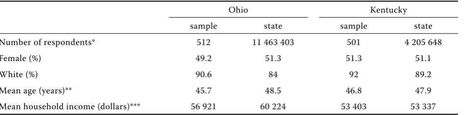
A total of 1013 consumers were included in the final sample. Descriptive statistics for the samples revealed a less than representative response for con-sumers older than 75 years and for males less than 35 years of age. For this reason, the sample responses were post-stratified by age and gender based on the 2007 decennial census.1 _{Table 1 reports several key} demographic features of the sample, which are then compared to the state-level statistics based on the 2007 census bureau data. Samples from both states are reasonably representative. Respondents in both states are older and have more representation of white individuals than the actual state average. The

Ohio sample had lower coverage of females while the Kentucky sample had slight over-coverage of females. Household income in the Ohio sample is lower than the state average and the Kentucky sample is almost identical to the state mean income.

The survey was designed to examine consumers’ general food purchasing habits, including where and how often they do their grocery shopping. The two key questions this study was interested in included a distance measure of local foods and the importance of being “local” for different food categories. The last section of the survey collected respondents’ demographic information.

ANALYSIS AND RESULTS

Results of this research are presented in two sec-tions: a descriptive statistics analysis gives a direct view of choices respondents indicated for the key variables of interest; a regression analysis reveals ad-ditional information on what factors may contribute to these choices.

Descriptive analysis

One of the questions in the first section of the survey asked respondents how many times they have purchased food in each of the following markets in the past 2 months: national grocery chains (e.g., Kroger), national “big box” retailers (e.g., Wal-Mart), locally owned groceries, convenience stores, spe-cialty food stores (e.g., organic), and farm or farmers’ markets. Figure 1 displays the result (N = 1013). For

Table 1. Sample descriptive statistics

Ohio Kentucky

sample state sample state

Number of respondents* 512 11 463 403 501 4 205 648

Female (%) 49.2 51.3 51.3 51.1

White (%) 90.6 84 92 89.2

Mean age (years)** 45.7 48.5 46.8 47.9

Mean household income (dollars)*** 56 921 60 224 53 403 53 337

* State population statistics are based on the 3-year estimates of the 2005–2007 American Community Survey (U.S. Census Bureau). Samples are post-stratified by age distributions and gender for each state.

** Mean age for consumers age 20 and older

*** Household income are presented in 2007 dollars after adjusting for inflation

1_{Additional variables could also be used in post-stratification. However, this makes the weighting process increasingly}

both national grocery chains and big box retailers, the two most commonly chosen categories are, in order, between 5 to 10 times and between 2 to 4 times. About 32% and 22% of the consumers shop in national grocery chains 5 to 10 times and 2 to 4 times in the past 2 months respectively. For national big box retailers, these numbers are 24% and 21%. Interestingly, for both types of stores, there are more than 10% of consumers who never shopped there during the past 2 months. If we combine both “none” and “once every 2 months”, there are respectively 20% and 30% consumers rarely shop in these two types of stores if at all.

For all other types of stores, the “none” category captures most consumers and the distribution of visitation to the other categories is similar across store types. If we classify those who visit one type of stores more than 5 times every 2 months as fre-quent visitors, for locally owned grocery stores these visitors account for 19% of the consumer body. For convenience stores this number is 13%; for specialty

food stores and farmers’ markets, the percentage of frequent visitors is 4% and 5% respectively. Not di-rectly shown in Figure 1, if one views locally owned grocery stores, specialty stores, and farmers’ markets as opportunities for selling locally grown foods, it is possible to calculate the potential customer base for these stores. Based on this sample, the percentage of consumers who visit any of these types of stores at least once over the past 2 months is 63%, which is consistent with findings in previous studies (e.g., Adams and Adams 2008). If visits to all stores by all individuals in the sample are summed up over the past 2 months, the percentage distribution of visits to each store is national grocery chains (41.22%), national big box retailers (29.95%), locally owned grocery stores (12.67%), convenience stores (9%), specialty food stores (2.69%), and farms or farmers’ markets (4.58%).

Figure 2 reports consumer responses to a question asking “what is the maximum distance (one-way) from your home that you would consider food to be locally

0 10 20 30 40 50 60 70 80 90

Percent

age

None Once 2–4 times

5–10 times 11–15 times >15 times

Figure 1. Distribution of grocery store visitors

National National Big Locally owned Convenience Specialty food Farm or grocery chain Box retailer grocery store store store farmers‘ market

0 10 20 30 40 50

25 miles 50 miles 75 miles 100 miles 200 miles 300 miles 500 miles within OH within the U.S.

Percentage

Categories

produced?” A miscommunication in the Kentucky questionnaire made this question unreliable for the Kentucky consumers. As a result, Figure 2 only reflects opinions of the Ohio respondents (N = 512). A vast majority of respondents (48%) indicated 25 miles is the limit greater than which they would unlikely consider as an appropriate travel distance for local foods.2 _{About 20%, 5%, and 12% of consumers} ac-cepted 50 miles, 75 miles, and 100 miles as their limit. This result not only provides more details about the definition of local food from consumers’ perspective than many previous studies, it also raises an impor-tant question, that is, whether the ad hoc measure of 100 miles held by many sources is indeed a suf-ficient measure of local foods for consumers. As is clearly shown by this study, at least 73% of consumers define local as less than 100 miles. In other words, only about 27% of consumers had 100 miles or larger as their acceptable travel distance for local foods. If producers or retailers are not aware of this gap between consumers’ actual understanding of local food distances and the generally believed measure utilized in current marketing programs, the implica-tions previously mentioned could occur, which may involve economic, ethical, and legal issues.

Other distance measures in Figure 2 are also use-ful. From 100 miles and above, it can be seen that when the distance measure increases, the percentage of consumer support decreases. From 100 miles to

200 miles, 300 miles, and 500 miles, the percentage of consumers to accept the measure decreases from 12% to 3%, 0.2%, and finally to 0. Therefore, it may be concluded that the recognition of local food decreases when the distance the products have to travel to reach consumers rises. Interestingly, there are consumers who believed products grown in Ohio (11%) and the U.S. (1%) can be called local. Clearly, for some Ohio residents, even products from within Ohio may come from well over 100 miles away. Similarly, for a product of the U.S., the 500 miles limit may easily be surpassed. It is likely that consumers who accepted Ohio or U.S. products to be local yet rejected a shorter actual distance attach additional values to these products when either the association with Ohio or the U.S. is mentioned (Darby et al. 2008).

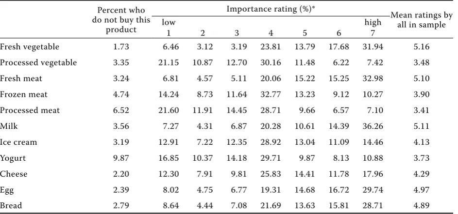
Table 2 depicts consumer ratings of the importance of local production to different types of food. Results presented use all 1013 sampled consumers in the two states. In the survey, respondents were given a Likert scale from 1 (low importance) to 7 (high importance) plus a “don’t know” option to mark their ratings of the importance of local across a variety of different food products. It is clear that consumers view the importance of local production very differently across product categories. As expected, respondents give the highest ratings of importance to fresh and perishable products. For each of the categories of milk, fresh vegetable, fresh meat, eggs, and bread, more than 25%

2_{This is a measure of what people would like to think of as local, not what they are willing to pay a premium for. In}

other words, this question asks respondents how close they would like to have food produced without tying it to the cost factor.

Table 2. Importance rating of “locally grown” for different food categories

Percent who do not buy this

product

Importance rating (%)*

Mean ratings by all in sample

low high

1 2 3 4 5 6 7

Fresh vegetable 1.73 6.46 3.12 3.19 23.81 13.79 17.68 31.94 5.16

Processed vegetable 3.35 21.15 10.87 12.70 30.16 11.48 6.22 7.42 3.48

Fresh meat 3.24 6.81 4.57 5.11 20.06 15.22 15.25 32.98 5.10

Frozen meat 4.74 14.24 8.73 11.64 32.77 13.23 9.12 10.27 3.90

Processed meat 6.52 21.60 11.91 14.45 28.71 9.66 6.57 7.10 3.41

Milk 3.56 7.27 4.31 6.87 20.28 10.61 14.39 36.26 5.11

Ice cream 3.19 12.91 7.22 12.35 28.92 13.04 11.09 14.46 4.13

Yogurt 9.87 16.85 10.37 14.18 29.71 9.87 8.13 10.88 3.73

Cheese 2.20 12.30 7.91 9.81 25.83 14.41 11.78 17.96 4.29

Egg 2.39 8.02 4.75 6.77 19.31 14.68 16.72 29.74 4.97

Bread 2.79 8.64 4.44 7.08 21.69 13.63 15.81 28.71 4.89

of those consumers who purchased this category gave the highest importance ranking for local production. For all remaining food categories, the most popular importance rating is 4 (moderate importance). The fact that for all food categories considered, the major-ity of consumers believed local production is either highly or moderately important further intensified the crucial role the “locally grown” feature may play in consumers purchasing decisions. The two product categories where local production received the most low importance ratings (rating 1) are processed meat (22%) and processed vegetable (21%).

Regression analysis

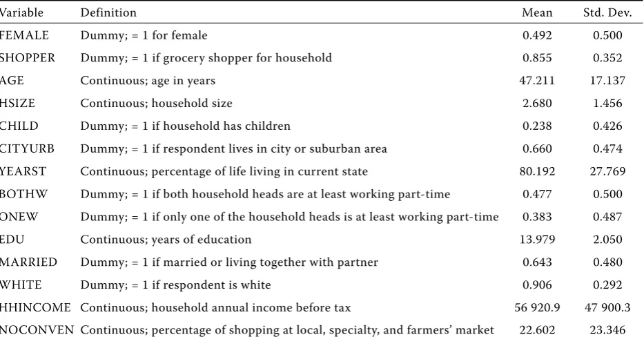
After knowing that different consumers may have different opinions on what could be called local, the analysis proceeds to examine what factors may contribute to these differences. An OLS estimate is conducted by regressing the chosen distance measures (in miles) on a set of consumer characteristics vari-ables also collected in the survey. Table 3 lists these variables and their descriptive statistics. Variable YEARST is calculated by taking the percentage of the number of years a person lives in the state (either OH or KY as self-identified by the respondent) of the person’s age. Variable NOCONVEN measures the percentage of grocery shopping done in a noncon-ventional store (e.g., local grocery, specialty store, or farm/farmers markets) for each individual respond-ent. The dependent variable DISTANCE takes the

value of the actual miles suggested by each option in the survey. For the 57 individuals who indicated “within Ohio”, their choices were treated the same as the 200 miles category. There were also a total of 5 respondents who said “within the U.S.”. This is difficult to merge with a specific mileage category given the potential diversity in distance suggested by the option. Since these individuals account for less than 1% of the data, they were not included in the regression analysis.

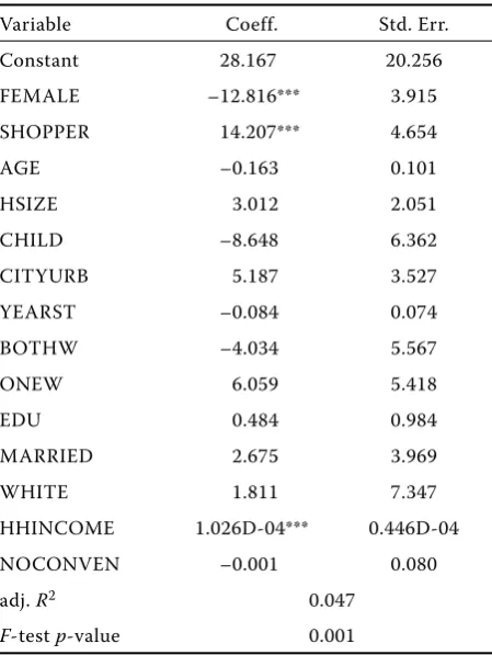
Using the Ohio sample, Table 4 gives the regres-sion result. Robust standard errors were obtained to guard against heteroskedasticity and the joint F-test suggested the model is significant. Although several variables are border-line significant, only three vari-ables are significant at the 10% significance level. Compared to males, female consumers appeared to be stricter in their required maximum allowed travel distance for local foods. Holding other factors constant, a female consumer’s “local radius” is about 13 miles shorter than a male consumer. Being the primary grocery shopper for the household seemed to loosen the standard. The result suggests that compared to a non-shopper, the primary shopper will allow local food to come from 14 miles further. Household income also has a positive impact on dis-tance. A quadratic income term was also attempted to capture any possible nonlinear impact but it was not significant. Based on the current model, every increase in household income by $10 000 will cor-respond to about one mile increase in allowed food traveling distance. Note that this result suggests that

Table 3. Descriptive statistics of variables used in regression analyses (N = 512)

Variable Definition Mean Std. Dev.

FEMALE Dummy; = 1 for female 0.492 0.500

SHOPPER Dummy; = 1 if grocery shopper for household 0.855 0.352

AGE Continuous; age in years 47.211 17.137

HSIZE Continuous; household size 2.680 1.456

CHILD Dummy; = 1 if household has children 0.238 0.426

CITYURB Dummy; = 1 if respondent lives in city or suburban area 0.660 0.474 YEARST Continuous; percentage of life living in current state 80.192 27.769 BOTHW Dummy; = 1 if both household heads are at least working part-time 0.477 0.500 ONEW Dummy; = 1 if only one of the household heads is at least working part-time 0.383 0.487

EDU Continuous; years of education 13.979 2.050

MARRIED Dummy; = 1 if married or living together with partner 0.643 0.480

WHITE Dummy; = 1 if respondent is white 0.906 0.292

those consumers who are more able to pay premium prices to receive local foods are actually less demand-ing that their food be produced nearby. Finally, in this model, the nonconventional shopping indicator did not appear to be significant in explaining the ac-ceptable distance local food may travel. Also, most consumer and household demographic variables were not significant at the 0.10 probability level.

The next step is to explain what factors may con-tribute to the different importance ratings for local production under different food categories. Initially, since the importance ratings are ordered data, an or-dered choice model is the appropriate specification. After removing observations with the “don’t know” answer (all but processed meat and yogurt had less than or about 3% of the sample choosing this option), an ordered logit model was conducted. However, sev-eral attempts were made and the models all failed to converge. This is likely caused by the many response categories allowed in the survey (1 to 7). A potential way to handle this problem is to combine the choices into fewer categories. Even after this transformation several product categories still didn’t have reasonable convergence. Most importantly, combining choices greatly reduced the richness of the data and defies the purpose of disaggregating the differences in im-portance rating. As a result, an OLS-type regression

was conducted for each food category after removing the “don’t know” observations. In this context, OLS regressions are not unsupported. The goal of the analysis is not to produce precise marginal effects of the explanatory variables nor offer predictions of choice probability. A regression model can be safely used to describe the qualitative impact of the regres-sors on the dependent variable.

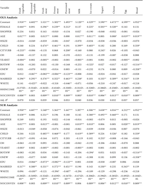
Table 5 presents the regression results of two sets of estimates and all standard errors used calculating the significance level are from the robust covariance matrix. The first approach used OLS models that regress the importance ratings for each food category separately on variables included in Table 3 plus an additional variable OH, which is a dummy variable equal one for Ohio residents. The second approach used is a group of seemingly unrelated regressions (SUR). They are conducted recognizing the pos-sibility that the rating decisions for different food categories may not be independent to each other. In order to avoid creating a large system of equations containing all food categories (which causes empiri-cal identification issues), four groups of models were identified. The first group contained 2 equations: fresh vegetable and processed vegetable; the second group was composed by fresh meat, frozen meat, and processed meat; the third group included dairy products: milk, ice cream, yogurt, cheese, and eggs; and bread is singled out as a group by itself (which generates identical result as in the single equation analysis). All models are significant.

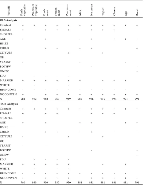
To facilitate interpretation and comparison, Table 6 summarizes the regression results. The “+” and “–” signs indicate the corresponding variable being posi-tive or negaposi-tive significant at least the 10% signifi-cance level. Insignificant variables are left blank. First, it is instructive to note that single-equation and SUR analysis generated highly consistent outcomes indi-cating the results are fairly robust across functional specifications. Second, although variable SHOPPER was not significant in either approach, the signs of FEMALE and HHINCOME are consistent with the implications in Table 4 -- The regression of distance on these variables showed that female consumers are more demanding than males that food be pro-duced nearby, while higher income households are less demanding of shorter food traveling distance. Variable FEMALE is consistently positive across all food categories when it’s significant. This shows that female consumers are more likely to give a higher importance rating for local production than males. Likewise, older consumers displayed significant positive coefficients in six food category models, and those who are married and who had children also

Table 4. Regression result to explain acceptable distance for local production

Variable Coeff. Std. Err.

Constant 28.167 20.256

FEMALE –12.816*** 3.915

SHOPPER 14.207*** 4.654

AGE –0.163 0.101

HSIZE 3.012 2.051

CHILD –8.648 6.362

CITYURB 5.187 3.527

YEARST –0.084 0.074

BOTHW –4.034 5.567

ONEW 6.059 5.418

EDU 0.484 0.984

MARRIED 2.675 3.969

WHITE 1.811 7.347

HHINCOME 1.026D-04*** 0.446D-04

NOCONVEN –0.001 0.080

adj. R2 _0.047

tended to display positive coefficient estimates. On the other hand, individuals with higher HHINCOME gave lower importance ratings in 10 of the product

categories, suggesting that they are more tolerant of nonlocal products. Although the level of consumer education was statistically significant only in four food

Table 5. Regression results to explain importance ratings of local production

Variable Fr e sh ve ge ta ble Pr o ce ss e d ve ge ta ble Fr e sh me at F ro zen me at Pr o ce ss e d me at Milk Ice c re a m Y o gu rt Che e se

Egg Bre

a

d

OLS Analysis

Constant 3.918*** 4.682*** 5.521*** 5.302*** 5.493*** 5.120*** 4.529*** 3.590*** 4.472*** 4.599*** 4.952***

FEMALE 0.444*** 0.091 0.296** 0.239** 0.212* 0.137 0.225* 0.503*** 0.320** 0.143 0.131

SHOPPER 0.234 0.051 0.163 –0.010 –0.154 0.027 –0.190 –0.048 –0.052 –0.081 –0.024

AGE 0.017*** 0.005 0.013*** 0.000 0.000 0.017*** 0.011*** 0.005 0.008* 0.019*** 0.019***

HSIZE –0.014 –0.049 –0.059 –0.081 –0.047 –0.070 –0.034 –0.038 –0.036 –0.003 –0.070

CHILD 0.240 0.224 0.474** 0.461*** 0.191 0.399** 0.403** 0.182 0.280 0.169 0.359*

CITYURB –0.233** –0.084 –0.135 0.068 0.208* –0.160 0.080 0.245* 0.026 –0.105 –0.043

OH –0.048 –0.157 0.132 0.005 –0.193 –0.013 –0.131 –0.199 –0.087 –0.038 0.088

YEARST –0.004** 0.002 –0.005** –0.002 –0.001 –0.005** –0.001 0.001 –0.002 –0.005** –0.002

BOTHW –0.026 –0.283 0.033 –0.130 –0.168 –0.253 –0.325* 0.027 –0.017 –0.127 –0.514***

ONEW 0.021 –0.070 0.022 –0.014 0.003 –0.151 –0.232 0.176 0.080 0.009 –0.358**

EDU 0.012 –0.067** –0.082*** –0.084*** –0.123*** –0.008 –0.041 –0.024 –0.041 –0.017 –0.028

MARRIED 0.296** 0.295** 0.376*** 0.352** 0.463*** 0.238* 0.103 0.335** 0.309** 0.316** 0.159

WHITE 0.141 –0.425** –0.022 –0.318 –0.446** –0.071 –0.056 –0.210 –0.247 –0.017 –0.218

HHINCOME –0.275D– 05** –0.354D– 05** –0.363D– 05** –0.454D– 05*** –0.350D– 05** –0.351D– 05** –0.328D– 05** –0.386D– 05** –0.258D– 05* –0.348D– 05** –0.184D– 05

NOCONVEN 0.008*** 0.003 0.009*** 0.010*** 0.009*** 0.005* 0.010*** 0.006** 0.013*** 0.010*** 0.009***

Adj. R2 _{0.070 0.026 0.059 0.046 0.053 0.040 0.036 0.030 0.032 0.057 0.057}

SUR Analysis

Constant 3.950*** 4.687*** 5.540*** 5.363*** 5.447*** 5.207*** 4.506*** 3.658*** 4.016*** 4.212*** 4.952***

FEMALE 0.438*** 0.086 0.251** 0.196 0.180 0.145 0.380*** 0.495*** 0.460*** 0.171 0.131

SHOPPER 0.249 0.051 0.193 0.022 –0.144 –0.014 –0.083 –0.079 0.015 –0.005 –0.024

AGE 0.017*** 0.005 0.013*** –0.001 –0.001 0.019*** 0.010** 0.004 0.005 0.020*** 0.019***

HSIZE –0.013 –0.049 –0.058 –0.074 –0.042 –0.061 –0.039 –0.030 –0.036 0.007 –0.070

CHILD 0.244 0.225 0.485*** 0.468*** 0.177 0.419** 0.389** 0.224 0.326* 0.182 0.359*

CITYURB –0.251** –0.091 –0.164 0.072 0.203 –0.119 0.102 0.255* –0.008 –0.166 –0.043

OH –0.063 –0.159 0.093 –0.051 –0.200 –0.042 –0.192 –0.206 –0.063 –0.070 0.088

YEARST –0.003* 0.002 –0.005** –0.002 –0.001 –0.005** –0.002 0.001 –0.001 –0.003 –0.002

BOTHW –0.083 –0.285 0.034 –0.083 –0.143 –0.204 –0.394* 0.051 0.025 –0.037 –0.514***

ONEW –0.023 –0.077 0.049 0.049 0.011 –0.118 –0.308 0.181 0.099 0.136 –0.358**

EDU 0.014 –0.066** –0.072** –0.082*** –0.122*** 0.001 –0.030 –0.030 –0.007 0.006 –0.028

MARRIED 0.317** 0.300** 0.331** 0.372*** 0.451*** 0.190 0.143 0.330** 0.235 0.343** 0.159

WHITE 0.094 –0.430** –0.121 –0.394* –0.407* –0.294 –0.189 –0.129 –0.298 –0.236 –0.218

HHINCOME –0.285D– 05** –0.349D– 05*** –0.354D– 05*** –0.459D– 05*** –0.347D– 05*** –0.475D– 05*** –0.306D– 05** –0.396D– 05*** –0.385D– 05*** –0.495D– 05*** –0.184D– 05

NOCONVEN 0.008*** 0.003 0.009*** 0.010*** 0.009*** 0.004 0.009*** 0.006** 0.012*** 0.010*** 0.009***

category models, EDUCATION uniformly exhibited negative coefficient estimates, suggesting that more highly educated consumers were less demanding that foods be produced nearby.

Overall, there exists a great deal of variation in which variable may be significant in which food category. Nevertheless, for the significant variables, they all have consistent signs across food categories

Table 6. Summary of importance ratings regression results

V

a

ri

able

Fr

e

sh

ve

ge

ta

ble

Pr

o

ce

ss

e

d

ve

ge

ta

ble

Fr

e

sh

me

at

F

ro

zen

me

at

Pr

o

ce

ss

e

d

me

at

Milk Ice

c

re

a

m

Y

o

gu

rt

Che

e

se

Egg Br

e

a

d

OLS Analysis

Constant + + + + + + + + + + +

FEMALE + + + + + + +

SHOPPER

AGE + + + + + + +

HSIZE

CHILD + + + + +

CITYURB - + +

OH

YEARST - - -

-BOTHW -

-ONEW

-EDU - - -

-MARRIED + + + + + + + + +

WHITE -

-HHINCOME - - - - - - - - -

-NOCONVEN + + + + + + + + + +

N 984 982 982 967 949 982 986 915 993 991 991

 SUR Analysis

Constant + + + + + + + + + + +

FEMALE + + + + + +

SHOPPER

AGE + + + + + +

HSIZE

CHILD + + + + + +

CITYURB - + +

OH

YEARST - -

-BOTHW -

-ONEW

-EDU - - -

-MARRIED + + + + + + +

WHITE - -

-HHINCOME - - - - - - - - -

-NOCONVEN + + + + + + + + +

except for CITYURB. Compared to rural residents, individuals living in cities or suburban areas tend to attach less importance to local production for fresh vegetable while the same group values local produc-tion more for processed meat and yogurt. Finally, as also suggested in Henseleit et al. (2007), consumers’ shopping habit may also be important factors in their choice of local foods. Variable NOCONVEN is significantly positive in all food categories except for processed vegetable. This suggests that consum-ers who shop at nonconventional stores more often tend to value local production more importantly for almost all foods they consume. It is quite likely that these consumers are self-selecting these nonconven-tional stores because they perceive that they better support their demand for local foods. Finally, it is important to note that the binary variable indicating Ohio consumers was not significantly different from zero in any food category model. This suggests that consumer preferences for local food appear to be stable across the two states.

CONCLUSION AND IMPLICATIONS

The demand for local food has been increasing at a striking pace over the past several years. Many food producers and retailers have engaged in local food production and marketing. As a result, not only shelf space in conventional grocery stores has been enlarged to accommodate more local foods, marketplaces specifically designed for local food such as Farmers’ Markets and CSAs have also seen tremendous growth. This poses an opportunity as well as a challenge. Despite the active demand and marketing activities, there is still paucity of studies on many issues surrounding local food. Relevant labeling laws are also severely lacking to address any dispute that may arise around local food. Using consumer data from two states in the United States, this study contributes to the understanding of two important questions: what is local and how important local production is for different food categories.

Results suggest that although the percentage of consumers shopping at nonconventional grocery stores is consistent with previous studies, instead of the commonly believed ad hoc distance of 100 miles, the majority of consumers (73%) have a much shorter perceived distance for food items to qualify as local. Consumer characteristics may help explain the difference in their acceptable distance measure. As for the importance of local production in dif-ferent food categories, fresh products in general receive higher importance ratings from consumers

than processed, frozen, or highly processed foods. Consumer characteristics and grocery shopping be-havior also have impact on the importance ratings. The impacts of these variables are consistent with those in explaining the actual distance measures.

Results found in this study have important im-plications for all stakeholders involved. For food producers, processors, and retailers, knowing how consumers view local food and its importance in their consumption choices is crucial to improve their ability to cover heterogeneous consumer groups and increase profit. A better understanding of the consumers may also keep these businesses away from potential ethical and legal issues that may rise given the current unclear and under-regulated local food sector. This is particularly important to small and medium-sized farms as they often struggle to sustain their operation and rely more heavily on the success of local food production and marketing as a niche. The prosperity of small and medium-sized farms is directly related to local economic development.

For consumers, a clear understanding of their needs will obviously be beneficial. Through carefully designed and defined local food marketing, consum-ers will be able to see more food varieties coming their way and more niche being fulfilled by produc-ers. They are all consumer benefit-enhancing. For policy makers, although flexibility in the definition may sometimes be desirable, the healthy develop-ment of the local food sector requires unambiguous guidelines. Regulations on issues such as what food can be claimed local, how they should be labeled and marketed, what monitoring tools should be in place to ensure authenticity, and how violators should be handled are all of great importance and should be developed soon to respond to the call of the current size of the local food sector. This study contributes to a timely discussion on these fronts.

REFERENCES

Adams D.C., Adams A.E. (2008): Availability, Attitudes and Willingness to Pay for Local Foods: Results of a Prelimi-nary Survey. Selected Paper. In: American Agricultural Economics Association Annual Meeting, Orlando, FL, July 27–29, 2008.

Alfnes F., Rickertsen K. (2007): Extrapolating experimental-auction results using a stated choice survey. European Review of Agricultural Economics, 34: 345–363. Brown A. (2002): Farmers’ market research 1940–2000: An

Brown C. (2003): Consumers’ preferences for locally pro-duced food: A study in Southeast Missouri. American Journal of Alternative Agriculture, 18: 213–224. Brown C., Miller S. (2008): The impacts of local markets:

A review of research of farmers markets and Commu-nity Supported Agriculture (CSA). American Journal of Agricultural Economics, 90: 1296–1302.

Carpio C.E., Isengildina-Massa O. (2008): Consumer Willingness to Pay for Locally Grown Products: The Case of South Carolina. Selected Paper. In: Southern Agricultural Economics Association Annual Meeting, Dallas, TX, February 2–6, 2008.

Coley D., Howard M., Winter M. (2009): Local food, food miles and carbon emissions: a comparison of farm shop and mass distribution approaches. Food Policy, 34: 150–155.

Crossroads Resource Center (2009): Direct Farm Sales Rising Dramatically, New Agricultural Census Data Show. Available at http://www.crcworks.org/press/ direct090214.pdf (accessed May 9, 2009).

Darby K., Batte M.T., Ernst S., Roe B. (2008): Decom-posing local: A conjoint analysis of locally produced foods. American Journal of Agricultural Economics, 90: 476–486.

Desrochers P., Shimizu H. (2008): Yes, We Have No Banan-as: A Critique of the ‘Food Miles’ Perspective. Mercatus Policy Series Policy Primer, No. 8. Mercatus Center at George Mason University, Arlington.

Dillman D.A. (2007): Mail and Internet Surveys: The Tai-lored Design. 2nd _{ed. Update John Wiley, Hoboken.}

Eastwood D.B., Brooker J.R., Orr R.H. (1987): Consumer preferences for local versus out-of-state grown selected fresh produce: The case of Knoxville, Tennessee. South-ern Journal of Agricultural Economics, 19: 183–194. Giraud K.L., Bond C.A., Bond J.J. (2005): Consumer

prefer-ences for locally made specialty food products across Northern New England. Agricultural and Resource Economics Review, 34: 204–216.

Govindasamy R., Italia J., Thatch D. (1999): Consumer attitudes and response toward state-sponsored agri-cultural promotion: An evaluation of the Jersey Fresh Program. Journal of Extension, 37: 60–69.

Hartman Group (2008): Consumer Understanding of Buy-ing Local. HartBeat Newsletter, February 27, 2008. Available at http://www.hartman-group.com/hart-beat/2008-02-27 (accessed May 8, 2009).

Henseleit M., Kubitzki S., Teuber R. (2007): Determinants of Consumer Preferences for Regional Food. Contrib-uted Paper. In: 105th European Association of Agri-cultural Economics, Bologna, Italy, March 8–10, 2007. Hu W., Woods T., Bastin S. (2009): Consumers’

accept-ance and willingness to pay for blueberry products with non-conventional attributes. Journal of Agricultural and Applied Economics, 41: 1–14.

Josling T. (2006): The war on terroir: Geographical in-dications as a transatlantic trade conflict. Journal of Agricultural Economics, 57: 337–364.

Lobb A.E., Arnoult M.H., Chambers S.A. (2006): Willing-ness to Pay for, and Consumers’ Attitudes to, Local, National and Imported Foods: A UK Survey. Report No. 2, June 2006, University of Reading.

LocalHarvest (2009): Community Supported Agriculture. Available at http://www.localharvest.org/csa/ (accessed May 9, 2009).

Lovenworth S.J., Shiner M. (2008): Protecting geographi-cally unique products. New York Law Journal, January 22, 2008. Available at http://www.deweyleboeuf.com/~/ media/Files/inthenews/ProtectingGeographicallyU-niqueProducts.ashx (accessed May 9, 2009).

National Restaurant Association (2009): Chef Survey: What’s Hot in 2009. Available at http://www.restau-rant.org/pdfs/research/2009chefsurvey.pdf (accessed May 9, 2009).

Packaged Facts (2007): Locally Grown Foods Niche Cooks up at $5 Billion as America Chows Down on Fresh! Available at http://www.packagedfacts.com/about/ release.asp?id=918 (accessed on May 9, 2009). Patterson P.M. (2006): State-grown promotion programs:

Fresher, better? Choices, 21: 41–46.

Schmit J. (2008): Locally Grown Food Sounds Great, but What does it Mean?” USA Today, October 28, 2008. Available at http://www.organicconsumers.org/articles/ article_15379.cfm (accessed May 9, 2009).

Smith A., MacKinnon J.B. (2007): The 100-Mile Diet: A Year of Local Eating. Random House Canada. Smyth J.D., Dillman D.A ., Christian L.M., O’Neill A .

(2010). Using the Internet to survey small towns and communities: Limitations and possibilities in the early 21st _{century. American Behavioral Scientist, 53:}

1423–1448.

Thilmany D., Bond C.A., Bond J.K. (2008): Going local: Exploring consumer behavior and motivations for di-rect food purchases. American Journal of Agricultural Economics, 90: 1303–1309.

Tranter R.B., Bennett R.M., Costa L., Cowan C., Holt G.C., Jones P.J., Miele M., Sottomayor M., Vestergaard J. (2009): Consumers’ willingness-to-pay for organic conversion-grade food: Evidence from five EU countries. Food Policy, 34: 287–294.

Tropp D. (2008): The growing role of local food markets: Discussion. American Journal of Agricultural Econom-ics, 90: 1310–1311.

Van Ittersum K., Meulenberg M.T.G., Van Trijp H.C.M., Candel M.J.J.M. (2007): Consumers’ appreciation of regional certification labels: A Pan-European study. Journal of Agricultural Economics, 58: 1–23.

Wal-Mart. (2008): Wal-Mart Commits to America's Farm-ers as Produce Aisles Go Local. Available at http:// walmartstores.com/FactsNews/NewsRoom/8414.aspx (accessed June 2, 2009).

Received: 23th _February

Accepted: 3rd _{April 2013}

Contact address:

Wuyang Hu, College of Economics and Management and College of Land Management, 1 Shizishan Street, Huazhong Agricultural University, Wuhan, Hubei Province, China, 630027