Design and Parametric Weight Optimization of Four Wheeler Lower Control Arm

3828

©IJRASET: All Rights are Reserved

Design and Parametric Weight Optimization of

Four-Wheeler Lower Control Arm

K. Sreekanth

_{, B. Anjaneyulu}

1, 2_{Mechanical Department, Gates institute of Technology}

Abstract: Suspension system of an automobile plays an important role in ensuring the stability of the automobile. Another major aspect of suspension system in passenger cars is luxury. A lot of research is going on in this direction, to further the development of independent suspension systems for automobiles. In the independent suspension system the control arm plays a major role. It is generally made of forged steel but this material is found to be excessively heavy in the current context of the quest for reducing the weight of the automobiles without any significant changes to design. In this task of designing the control arms with alternative materials, Computer Aided Engineering (CAE) software being extensively used to perform the topology optimization. The main objective of this study is to reduce the weight of the lower control arm of independent suspension by using topology optimization and material optimization. Static loads were taken into consideration and analysis is done for two different models viz. the existing model and an optimized model developed by topology optimization. Static structural analysis s& modal analysis of lower control arm is carried out by using HYPERWORKS. The obtained results of existing model are compared with the optimized model and their weights are calculated for two different materials. The best model from this study is proposed based on the topology and material optimization.

Keywords: Suspension system, Computer aided Engineering

I. INTRODUCTION

A. Introduction to Suspension System

In automobiles, a double wishbone suspension is an independent suspension design using two wishbone-shaped arms to support the wheel as shown in Fig 1.1.Double wishbones provide more stability to wheel movements at high speeds which reduces camber angle as the wheel moves up and down over uneven surfaces. Wishbones can be very easily adjusted as every joint can be removed for optimal wheel movement. During the actual working conditions, the maximum load is transferred from upper wishbone arm to the lower arm which may cause failure and bending of lower wishbone arm either at the ball joint location or at control arm because of high impact loads that are could be produced by road conditions. Such failure should be avoided to ensure the reliability of the suspension system and the automobile.

Fig 1.1 Suspension System

Double wishbone suspension system is one type of independent suspension system which consists of two lateral control arms namely upper and lower arm. The control arm is nearly flat and roughly triangular member that pivots in two places. The broad end of triangle is attached at the frame and pivots on bushing. The Lower control arm is also called as A-arm. Control arms can be used in an all-wheel independent suspension system.

3829

©IJRASET: All Rights are Reserved

The lower control arm is one of the major parts of the front suspension system which controls the wheel trace and transmits the load on the wheel by the road to other parts of the car. When the car runs on the road, the lower control arm is subjected to complex loads that constantly change with time. Thus, the mechanical performance, usually relating to strength and stiffness are critical to the safety and reliability of the car.

The main functions of control arm are:

1) To form a rigid connection between the chassis and wheel hub, to which wheel is attached. To allow the wheel, the required degrees of freedom for proper steering and suspension abilities.

2) To support the spring and dampers, which form the major components for shock absorbing.

To do these functions properly the control arm needs to be sufficiently strong. Depending upon the position of the control arm, there are mainly two types of control arms Upper and lower control arm. The springs and shock absorbers are supported between these arms.

B. Methodology

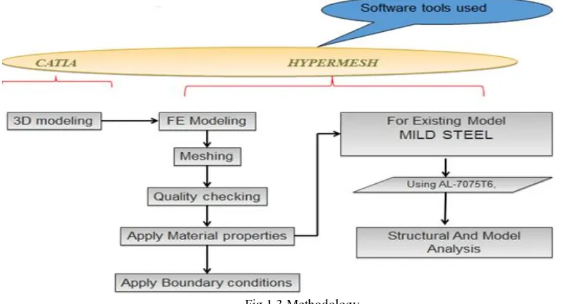
In methodology, the steps involved in this study are discussed as shown in fig 1.3. Mainly two steps are there. First is design the component and second is analysis with meshing. Design is done in 3D modelling CATIA, meshing and analysis is done in HYPERMESH.

Fig 1.3 Methodology

Initially we have developed the model using CATIA, based on an existing geometry. CATIA model is meshed with the help of HYPERMESH and analysis is carried out for two different materials (base material: Mild steel and the alternative material used in this study: Aluminum7050 T6) using HYPERWORKS.

3830

©IJRASET: All Rights are Reserved

C. Objective

The lower control arm of a four wheeler of “HZJ 75”is chosen for the present study. The details of the geometry are taken from the existing component and it is developed by the commercial modelling tool “CATIA”. The developed lower control arm consists of three holes, one each and the three ends of the arm. At one end the arm is fixed to the wheel hub and other two endsare connected to the chassis and the steering link.

The main objective of this study is

1) To reduce the weight of the lower control arm by using topology optimization and material optimization.

2) Static loads were taken into consideration and analysis is done for two different models viz. the existing model and an optimized model developed by the topology optimization.

3) Static structural analysis & modal analysis of lower control arm is carried out by using HYPERWORKS.

4) The obtained results of existing model are compared with the optimized model and their weights are calculated for two different materials.

5) The best model from this study is proposed based on the topology and material optimization.

II. LITERATUREREVIEW

In automotive industry simulation-based improvement of models has been used for a variety of applications. In the study of Xue Guan Song et al.(2010), based on the FEM analysis, both the response surface model(RSM)and Kriging model are used to optimize an ADI upper control arm, where the weight of the upper control arm is considered as the design objective, and the maximum allowable vonmises stress is the constraint objective. The initial FEM analysis shows the stress distribution and maximum stress on the upper control arm under a very severe loading condition. And, by virtue of the result of FEM analyses, fifty simulations with six design variables are performed for RSM and Kriging model to construct the approximation of the weight and maximum stress to obtain the optimum result. The optimized results obtained by using RSM and KRG are confirmed by a verified FEM analysis. In addition, a fatigue analysis is carried out to verify the durability of the final design. Suspension system of an automobile plays an important role in ensuring the stability of the automobile. Although it has been achieved to a considerable extent, another major aspect of suspension system in a passenger car is luxury. A lot of research is going on in this direction, which resulted in the development of independent suspension system. Control arm plays a major role in independent suspension system. It is generally made of forged steel which has considerable disadvantages such as weight, cost etc. P. Nagarjuna et al. (2012), presented the development of sheet metal control arm, which has many advantages over forged metal.

Stability, road handling and comfort of vehicle depend on optimum design of suspension system. Mostly all passenger cars and light trucks use independent suspension system because of inherent advantages over rigid suspension systems. Double wishbone system which is also called as Short Long Arm system consists of upper and lower wishbone arms. While actual running condition forces like braking, cornering and vertical loads are taken by lower arm of suspension system, hence probability of failure of lower arm under these forces is more. Also this component is subjected to road irregularities, hence its dynamic behaviour need to be understood. The study conducted by Vinayak Kulakarni et al. (2014) deals with calculating the forces acting on lower wishbone arm while vehicle is subjected to critical loading conditions (Braking, Cornering and Descending though slope). Suspension geometry and suitable materials for the suspension arm have been identified. Lower arm suspension has been modelled using Pro-Engineer. Vonmises stress –strain is carried out in order to find out maximum induced stress and strain, while modal analysis is done for finding out natural frequencies and mode shapes of component are analysed in the study. These analyses were carried using Altair Hyper works and solver used is Radios. From the analysed results, design parameters were compared for two different materials and best one was identified. From result obtained it was found that existing design was safe and was somewhat overdesign. So in order to save material and reduce weight of component, Topology optimization analysis is carried out in Hyper works which yielded in optimized shape.

3831

©IJRASET: All Rights are Reserved

In automobile components of vehicles suspension system is one of the important components. This suspension system directly affects the performance, safety and noise level. A good suspension system is also crucial for the comfort and safety of the passengers. Lower control arm is a part of suspension system; this transmits all the forces between road and body and also absorbs the vibrations. Under static load conditions structure optimization techniques have been commonly used in automotive industry to improve the performance and reduce the weight of latest cars. But static load conditions are not the actual operational load for all the components of suspension system which are subjected to complex loads varying with time, particularly lower control arm. Sagar Darge et al. (2014) conducted topology optimization of lower arm suspension of double wishbone suspension by using finite element analysis. Design of the lower arm suspension is done in Uni graphics. Analysis is done in Altair Hyper Works and solver used is Abacus. In first stage of analysis area of maximum stress is recognized. In second stage it was attempted to improve the structural strength and reduce the stress using topography optimization approach in Hyper Works. Stiffness is improved for a lower arm suspension. The study of A.S. Todkar et al. (2013), was focused on stress strain analysis of lower control arm. The wishbone control arm is a type of independent suspension used in motor vehicles. The general function of control arms is to keep the wheels of a motor vehicle from uncontrollably changing the direction when the road conditions are not smooth. The control arm suspension normally consists of upper and lower arms. The upper and lower control arms have different structures based on the model and purpose of the vehicle. By many accounts, the lower control arm is the better shock absorber than the upper arm because of its position and load bearing capacities. It has an “A” shape on the bottom known as wishbone shape which carries most of the load from the shock received. The lower control arm takes most of the impact that the road has on the wheels of the motor vehicle. It either stores that impact or sends it to the coils of the suspension depending on its shape. During the actual working condition, the maximum load is transferred from upper wishbone arm to the lower arm which creates possibility of failure in the arm. Similarly, impact loading produces the bending which is not desirable. Hence it is essential to focus on the stress strain analysis study of lower wishbone arm to improve and modify the existing design. The present study will contribute in this problem by using finite element analysis approach.

III.MODELLING

A. Introduction to CATIA V5

The full form of CATIA is computer aided three dimensional interactive applications and it was developed by Dassault system, in France

The CATIA is a powerful CAD/CAE/CAM tool for product life cycle management. It is easy to because of its flexibility and its versatility enables designing of complex geometries as well as quick re-designing of available geometries. And it is also improves the innovative design concepts and gives the best design strategy, better productivity and creativity. It helps in creating the product from concept generation to the final product with in the given span of time with best design.

In CATIA, we have different types of workbenches. A workbench means definite environment which involves the set of tools and these tools are utilized to perform the best design within a particular area

The basic workbenches in CATIA are 1) Part design workbench

2) Wire frame and surface design workbench 3) Assembly design workbench

4) Drafting workbench

5) Generative sheet metal design workbench

B. Basic Functions in “CATIA V5”

1) Sketcher: CATIA sketcher tools primarily draft a rough sketch following the shape of the profile. The objects created are converted into a proper sketch by applying geometric constraints and dimensional constraints. These constraints refine the sketch according to a rule. Adding parametric dimensions further control the shape and size of the feature. Line, rectangle, palette, constrain, dimension modification, and text etc., are used as one of the feature creation tools to convert the sketcher entity into a part feature.

3832

©IJRASET: All Rights are Reserved

b) Assembly Design: It allows the design of assemblies with an intuitive and flexible user interface. As an accessible workbench, Assembly Design can be used in conjunction with other current companion products such as Part Design and Generative Drafting.

c) Interactive Drafting: It is a new generation product that addresses two dimensional design and drawing production requirements. Interactive Drafting is a highly productive, spontaneous drafting system that can be used in a standalone 2D CAD environment within a backbone system. It also expands the Generative Drafting product with both integrated 2D interactive functionality and an advanced production environment for the dress-up and explanation of drawings. This provides an easy and smooth evolution from 2D to 3D –based design methods.

2) Basic Characteristics of CATIA

a) Feature based modelling: The component design involves a number of stages in the CATIA. If we change any individual feature in one stage, it will automatically reflect into the final product and it is modified according to this. We don’t need to go back for the modifications. So it is a flexible and user friendly tool.

b) Parametric Modelling: It is an ability to utilize the standard properties or parameters for the size and shape of the geometry. We have flexibility to modify the size of any feature at any stage of design process.

c) Bidirectional Associatively: If any modifications are made in any one work bench and it will automatically reflects to all work benches where the model is designed.

CATIA V5 is totally compliant with windows presentation standards. CATIA V5 provides unique two way interoperability with older versions of the same. As an open solution, CATIA includes interfaces with the most commonly used data exchange standards.

C. Catia V5 R20

The 3D model of the double wishbone control arm is designed by using CATIA V5 R20.This release of CATIA, extends the power of leading edge engineering practices to include relation design, which results in

1) Higher quality design, the first time 2) More opportunities for innovation

3) Fewer engineering changes later in the design cycle

a) CAITA V5 R20 portfolio brings business values in the following areas i) Power major product programs

ii) Process expertise

iii) World class PLM(Product Lifecycle Management) iv) Proven openness and standards support

D. Design of Lower Control Arm

As we know that the lower control arm is very important that and it should have proper stiffness and strength characteristics for the safety of a vehicle, while maintaining light weight. The details of the geometry are taken from the existing component and it is developed by the commercial tool CATIA.

After opening the CATIA, one plane is selected and the sketcher workbench is activated to develop 2D model based on the dimensions.After this the sketcher is closed 3D model is created using suitable commands.

3833

©IJRASET: All Rights are Reserved

Before starting the geometric modelling of the lower control arm, the origin is assumed. Based on the origin we can develop 2D sketches of each of the parts of the model in the sketcher as shown in fig 3.1 and with the use of suitable commands convert 2D sketchers into 3D solid components using “EXIT WORKBENCH”.

E. Modelling Procedure

In the CATIA development environment, mechanical design s selected, and in that part design is selected to design the lower control arm, this is shown in fig3.2

1) Select part design in CATIA

Start →Mechanical design →Part design →Enter Name (Control Arm)

Fig3.2: Part design selection in CATIA

Shape of the lower control arm is designed by the dimensions used by Kulakarni et al. (2014) with the use of sketcher, line, arc, etc. Shape of the lower control arm is shown in fig 3.3.

Fig3.3: Control arm of 2d profile

After completion of shape, thickness of the control arm is given as 90mm thickness this is gives a rough shap of the control arm shown as in fig 3.4

Pad→ Select type as dimension→ specify thickness→ ok

3834

©IJRASET: All Rights are Reserved

2) Create hole on control arm profile2d profile of hole

3) Pocket create on control arm pocket→ select type as up to last → ok.

Control arms usually come in different shapes. To design the ford car control arm material is removed from the two sides of the control arm as shown in figure 3.5.

Fig 3.5: Profile of hole

Control arm has three holes at the three ends. Two holes are parallel to each other. These are attached to the wheel hub. One hole is attached to the chassis. These holes are created using pocket option as shown in fig3.6.

4) Pocket create on control arm

Pocket→select types as dimension→ specify thickness.

Fig 3.6: Profile of hole

The ends of the control arm at this stage are angular. To design the smooth and rounded ends of required shape for the control arm, the pocket option in selected once again to remove the sharp edges as shown in fig 3.7, then the final component of lower control arm is designed.

5) Create pocketon control arm profile

Pocket→ select type as dimension →specify thickness

3835

©IJRASET: All Rights are Reserved

IV.MESHING

A. Import File in Hypermesh

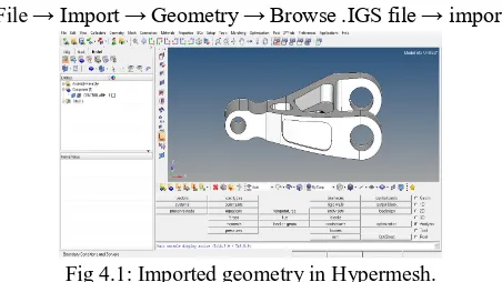
The details of the geometry are taken from an existing component and the 3D model is developed by the commercial tool “CATIA” as described above and the file is saved in step file. After developing the CATIA model, it is exported to HYPERMESH. The figure 4.1 shows the imported file from CATIA.

1) Import the CAD model into Hypermesh V13.

File → Import → Geometry → Browse .IGS file → import

Fig 4.1: Imported geometry in Hypermesh.

B. Meshing

Steps involved in meshing of the geometry using Hypermesh are selection of mesh type, meshing method and type of elements used in the mesh as shown in figure4.2.

Mesh Type: 3D mesh

Mesh Method: Volume Tetra Mesher Mesh Element: Tetrahedral

Mesh → 3D → Tetra Mesh → Volume Tetra → Element Size → 10 → Mesh

Fig 4.2: Meshing component

C. Finding Free Edges

In addition to the node connectivity problems, there could also be free edges in the generated mesh. The presence of free edges and T edges between the nodes and elements should thus be checked after meshing. If there are any free edges and T edges on the component, remeshing may be required to eliminate the free edges. The free edges in hypermesh could be found using Shift+F3 option. Free edges are shown in figure 4.3.

 Tool→ edges→ elements→ displayed→ find edges

3836

©IJRASET: All Rights are Reserved

D. Removing Edges

If there are any spurious edges that are created these edges are saved into temp file. From the temp file elements related to free edges can be found using shiftF3 and they can be removed. The final component, the control arm with the mesh is shown in figure 4.4.

Figure 4.4: Final meshed model E. Elements Checking

If there are no free edges on the component, then it is required to find the failure elements using “tap collapse” option. If there are any failure elements on the component we have to modify them using avilable options in hypermesh (Split surface line, replace point etc.,) to get better results. The tap collapse could be found in hypermesh using Shift+F10 option. To get the quality analysis check the below functions as shown in figure 4.5.

Tool→ check elements→ 3D→ warpage→ connectivity→ check.

The elements are treated as failed elements if they do not conform to the following criteria: Tet collapse<0.1

Aspect < 5 Jacobian < 0.7

Figure 4.5: Elements checking in hyper mesh

F. Calculate the Number of Nodes and Elements

If there are no free edges and no failure elements on the component then the meshing is ready to do analysis. Before that the number of nodes and elements present on the existing model is calculated using tool option.The total number of nodes are shown in figure 4.6

Figure 4.6: No of nodes and elements displayed option in Hypermesh

3837

©IJRASET: All Rights are Reserved

G. Creating Rigid

Lower control arm has three holes. Force and constraints are applied at the holes to apply the loads rigids are created and given the two different colours. Two holes are attached to the wheel hub and remaining hole is attached to the chassis as shown in fig 4.7.

Go to 1D→rigids→dependent→muliple nodes→ select node→ by face→ create→ Return

Fig 4.7: Creating rigids.

H. Constraints

In the control arm one end is fixed and other end is free. Two parallel holes which are in green colour are fixed in all degrees of freedom constraining of control arm is shown in fig4.8.

Fig 4.8: Constraints I. Apply the Loads

The force is analytically calculated. This force is applied at the remaining hole which is in yellow colour. Force is applied in downward Z-direction is shown fig 4.9.

Analysis→ Loads→ Force→ Select the shell elements→ Enter pressure value 0.0377MPa→ Create→ Return.

Fig 4.9: Applying force on control arm in z-direction

J. Materials Properties

3838

©IJRASET: All Rights are Reserved

Table 4.1: Material properties

Mechanical properties Mild steel AL-7075T6

Young’s Modulus ( MPa) 210000 71700

Poisson’s Ratio 0.3 0.33

Density (kg/m3) 7850 2890

Yield Stress (MPa) 350 503

In the material collector, enter the material type as ISOTROPIC and card image as MAT1 and click on the create/edit option shown in Figure 4.10.

Figure 4.10: Mild steel collector

K. Mechanical Properties of Mild steel

After assigning the material collector, it is necessary to enter the material properties like E (young’s modulus), G (modulus of rigidity), NU (Poisson’s ratio) and RHO (Density) in the property table shown in Figure 4.11.

Figure 4.11: Mild steel material properties

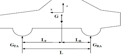
L. Load Calculations

Four wheeler vehicles have many geometric dimensions. These dimensions are measured from the centre of gravity of the vehicle. Some of the geometric parameters which are used in the load calculations are shown in below fig 4.12 and defined in Table 4.2.

3839

©IJRASET: All Rights are Reserved

Table 4.2: Specifications of the vehicle

Parameters Descriptions

B Width of vehicle

B Front axle track width

H Vehicle Height

L Length of centre of gravity

L Length of vehicle

LF Distance from front axle to centre of gravity

LR Distance from rear axle to centre of gravity

In this study, control arm is taken from the four wheeler vehicles of Ambassador, ford cars. Specifications of these cars are shown in below

Mass of vehicle (M): 3050 kg.

Front axle track width (B):1.67m-1670mm Height of centre of gravity (H):1.16m-1160mm Friction co-efficient b/w the road and tire (FS):0.6

Static load on front and rear axle load ( GFa/GRA):44/56

Height of vehicle (h):2220mm

Area a moment of inertia of the cross section (I): 4800mm4

Wheel base of vehicle (L):2900mm

Distance from front axle to C.G (LF):1624mm Distance from Rear axle to C.G (LR):1276mm Radius of turn (or) curvature(R):100mm

The angle of upper suspension arm (α):11

M. Static Axle Loads

When the weight of vehicle is at the centre of gravity then the loads are calculated by using the fig 4.13

Figure 4.13: Static axle loads on the vehicle

G= m.g

The loads on the front and rear axles are found by using the equilibrium equations: G = mass .gravity

G= 3050*9.81

Weight (G) = 29920.5N.

GFA = , =13165.02 N

GRA = , = 16755.48N

Static load on one wheel of the front axle is

GFAw = = = 6582.51N

3840

©IJRASET: All Rights are Reserved

All calculations presented are based on the main assumption that the chassis of the car under consideration is rigid. Calculation of the loads at each wheel in different operating conditions will be discussed for the rest of this section:

1) The vehicle braking on level ground 2) The vehicle at the instant of cornering 3) The vehicle downhill grade

4) The vehicle at the instant of braking on a downhill grade. a) CASE:-1.The vehicle braking on level ground :

Figure 4.14: Forces acting on a vehicle during braking

The car is under negative acceleration as show in figure 4.13, an inertial reaction force denoted by (G/g.a) acting at the centre of gravity opposite to the direction of the acceleration. During the vehicle decelerates, load is transferred from the rear axle to the front axle.

By considering the equilibrium of moments about the front and rear tire-ground contact points, the normal loads on the front and rear axle are,

GFAdyn = , = 13176.3172 N.

GFAdyn = , = 16744.182 N

The transferred load to the front axle is found from the following equation GT = GFAdyn - GFA, 13176.3172-13165.02 = 11.2972 N.

b) Case2: The vehicle at the instant of Cornering: (Lateral Load Transfer on the Banking)

Figure 4.15: Forces acting on a vehicle during cornering

The centrifugal force which results from the speed V , the radius of the bend R and the total weight of the vehicle is;

FC =

Fc = Centrifugal force V = velocity

3841

©IJRASET: All Rights are Reserved

GRS dyne =

GRS dyne =

GRS dyne = 38495.12982N

GLS dyne =

GLS dyne =

GLS dyne = -8574.629N

Transferred load from the left side to the right side of the vehicle while cornering

GC = GRS dyne -

GC =

GC =23534.879N.

c) Case: 3 The vehicle on a Downhill grade

Figure 4.16: Forces acting on a vehicle on a downhill grade

A negative grade causes load to be transferred from the rear to the front axle. On roads, the grade angle occasionally reaches 10 to 12 per cent,

The major external direction, the aerodynamic resistance Ra, rolling resistance of the front and rear tires Rrf and Rrr are neglected for

this case,

The dynamic loads on the front and rear axle are determined by summing moments equilibriums

GFA dyne =

GRA dyne =

GFA dyne = =15146.0146N

GRA dyne = = 14163.99442N

Transferred load from rear axle to front axle is GT = GFA dyne - GFA

GT = 15146.0146-13165.02

GT = 1980.9946N.

3842

©IJRASET: All Rights are Reserved

Figure 4.17: Forces acting on a vehicle braking on a downhill grade

The dynamic loads on the front and rear axle are determined by the summing moments equilibriums

GFA dyne =

GFA dyne =

GFA dyne = 71290.258N

GRA dyne =

GRA dyne =

GRA dyne = 69397.4878N.

GFAw = , = =35645.1291N.

The braking inertia force is: FA = m .a

The aero dynamic forces produced on a vehicle arise from two sources,from (or pressure) drag and rolling resistance of the tires. Drag is the largest and most important aerodynamic force. The aerodynamic drag is

FD = CD.A * *V2

FD = 0.32*3.482*1.288/2*33.332

FD =797.14117

The drag coefficient, CD is determined empirically for the car. The frontal area, A is the scale factor taking into account the size of

the car. The frontal area of the vehicle in range of 79-84% of a car calculated from the overall vehicle width and height. The frontal area %80 of area is

A = 0.80.b.h, A = 0.80*1.961*2.22 A = 3.482m

The aerodynamic force is assumed to be acting on the canter of the vehicle cross-section area

Hh =

Hh =

Hh = 1.11m

The other major vehicle resistance force on level ground is the rolling resistance of the tires by the equation FR = G.fR. Cosα

FR = 29920.5*0.015*cos (11)

FR = 440.561N.

3843

©IJRASET: All Rights are Reserved

O. Analysis

Whenever meshing is completed the component is ready for analysis. The structural analysis and Modal analysis carried out in ALTAIR Optistruct. The structural analysis carried out for finding the stresses and displacement of component. The modal analysis carried out for dynamic properties of component under vibrational excitation.

1) Structural Analysis

To determine the vonmises stresses and displacement of the model linear static structural analysis is selected as the objective. In static structural analysis the single point constraint (SPC) and the applied loads are given as inputs. The analysis is carried out by Optistruct solver gives an output of stresses and displacement values as shown in Figure 4.18.

a) Create a load collector name as SPC(Single Point Constraint)

Analysis→ Constraints→ Select nodes→ Select Degree of freedom→ Create→ Return.

Figure4.18:Creation of fixing constraints for structural analysis

b) Solve the analysis

Analysis→ Optistruct→ Select the output directory→ run options as analysis→ Optistruct

Figure 4.19: Solver setup for structural analysis

2) Modal Analysis: In Hyperworks the static structural analysis is converted into normal mode analysis by the using of card image “EIGRL” as shown in Figure4.20. In normal mode analysis the card image “EIGRL”, single point constraint (SPC) and the applied loads are taken as input. The analysis is carried out by Optistruct solver and gives an output of frequency range and mode shapes of the model.

Create load collector name as modal and card image as EIGRL

Collectors→ Load collector→ Name as modal→ card image as EIGRL→ Create/Edit

3844

©IJRASET: All Rights are Reserved

a) Solve the Analysis

Analysis→ Optistruct→ Select the output directory→ run options as analysis→ Optistruct

Figure 4.21: Solver setup for modal analysis

V. RESULTS

A. Static Structural analysis

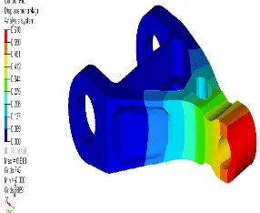
Lower control arms are generally made of mild steel due to their high compressive strength, wear resistance, excellent machinability, low cost, etc. First simulation is performed by taking the material of the control arm to be mild steel. The lower control arm behaves like a cantilever beam at the one hole side is fixed and two holes side is free. From the fig6.1 it is clear that maximum displacement occurs at the free end.

Figure 5.1: Displacement for mild steel reference design

Based on the given loading conditions the model behaves like a cantilever beam. For cantilever beam the maximum bending stresses is developed at fixed support. The von Mises stress distribution of mild steel of lower control arm is shown in the figure 5.2

Figure 5.2: Vonmises stress for mild steel reference design.

3845

©IJRASET: All Rights are Reserved

Figure 5.3: Displacement for aluminium-T6design.

Figure5.4: Vonmises stress for aluminium-T6design

B. Optimized Model

1) Mild Steel: After completion of topology optimization First simulation is performed by taking the material of the control arm to be mild steel. From the fig6.5 it is clear that maximum displacement occurs at the free end. The maximum displacement of mild steel material is 0.609mm

Figure 5.5: Displacements for mild steel optimize model design.

The optimized design is having the less stress when compare with the existing design as shown in Figure6.6. The vonmises stress of the optimized model is 63.527mm.

Figure 5.6: Vonmises stresses for mild steel optimize model design.

3846

©IJRASET: All Rights are Reserved

Figure 5.7: Displacement for aluminium-T6 optimize model design

For cantilever beam the maximum bending stresses is developed at fixed support. The von Mises stress distribution of lower control arm is shown in the figure6.8. The maximum displacement of lower control arm is 62.940mm.

Figure 5.8: Vonmises stresses for aluminium-T6 optimize model design.

C. Discussion of Structural Analysis

The results of the structural analyses conducted for four different cases are summarized here. The maximum von Mises stresses and maximum displacements for each of two materials are as shown in the table 6.1, and they are also graphically presented in graph6.1 and6.2 respectively.

Final results

Materials

Base design Optimized design

Displacement (mm) Vonmises Stress (MPa) Displacement (mm) Vonmises Stress (MPa)

Mild steel 0.618 100.51 0.609 63.527

Al-T6 1.813 99.717 1.026 62.94

Table 5.1: Results obtained from the static structural analysis

1) Comparison of Stress: As was discussed already the comparison of the maximum stress across the four different cases considered here see Table6.1 shows that AluminiumT6 alloy after optimization gives least maximum stress while mild steel before optimization gives highest maximum stress. However, considering the weight of the lower control arm, AluminiumT6 alloy gives the least weight with the choice of given its low density.

MILD

STEEL ALT6

BASE MODEL 100.51 99.717

OPTIMIZE MODEL 63.527 62.94

100.51 99.717

63.527 62.94

0 20 40 60 80 100 120 STRESS(M Pa) BASE MODEL OPTIMIZE MODEL

3847

©IJRASET: All Rights are Reserved

2) Comparison of Displacement: A comparison of maximum deflection in all the cases considered here shows that AluminiumT6 alloy before optimization gives largest deflection. Also, Mild steel is having the less displacement because of its density.

mild steel Al t6

Base model 0.618 1.813

optimize model 0.609 1.026

0.618

1.813

0.609

1.026

0 0.5 1 1.5 2

Base model

optimize model

Graph 5.2: Displacement for base model and optimize model D. Modal Analysis

In this analysis, we determine the vibration characteristics and it is also used to calculate the natural frequencies at corresponding mode shapes. Various mode extraction methods are available. The required boundary conditions are, two holes was fixed in all degrees of freedom and the material properties was given for extracting the first three mode shapes of control arm are shown below. 1) Mode Shapes of existing model – Mild steel Mode1: The different mode shapes and its natural frequencies of the base model

with mild steel are shown in Figures 6.9 – 6.11.

Figure 5.9: Mode-I for mild steel reference design.

Figure 5.10: Mode-II for mild steel reference design.

3848

©IJRASET: All Rights are Reserved

2) Mode Shapes of existing model – aluminium-T6: The different mode shapes and its natural frequencies of the base model with aluminium –T6 are shown in Figures 6.12 – 6.14.

Figure 5.12: Mode-I for aluminium-T6design

Figure 5.13: Mode-II for aluminium-T6design

Figure 5.14: Mode--III for aluminium-T6design

E. Modal analysis Results

Materials Base design Optimized design

Mode-1 Mode-2 Mode-3 Mode-1 Mode-2 Mode-3

Mild steel 3.406 9.188 9.464 1.329 2.900 3.595

Al-T6 3.258 8.810 9.124 4.027 8.839 9.123

3849

©IJRASET: All Rights are Reserved

1) Graph: Based on the above results we draw the graph between mild steel alt6 model by comparing for base model frequencies as shown in below.

MODE-1 MODE-2 MODE-3

MILD STEEL 3.406 9.188 9.464

ALT6 3.258 8.81 9.124

3.406 9.188 9.464 3.258 8.81 9.124 0 2 4 6 8 10

BASE MODEL

Graph: 5.3: Frequency modes for base model

2) Graph: Based on the above results we draw the graph between mild steel alt6 model by comparing for optimize model frequencies as shown in below.

MODE-1 MODE-2 MODE-3

MILD STEEL 1.329 2.9 3.595

ALT6 4.027 8.839 9.123

1.329 2.9 3.595 4.027 8.839 9.123 0 2 4 6 8 10 MILD STEEL ALT6

Graph: 5.4: Frequency modes for optimize model

F. Calculation of Weight

The main objective of this study is to reduce the weight of the lower control arm using topology optimization and material optimization. In material optimization, it is necessary to introduce the materials having good mechanical properties like high strength to weight ratio. Mild steel and Aluminium alloy 7050T6 are used for this study to reduce the weight of the component. To calculate the weight of the model, use tool option displayed in Hyperworks. In tool option, click on the mass calculation option and select the all displayed elements to calculate the weight of the model as shown in Table6.3

Materials Base design weight in(kg) Optimized design weight in(kg)

Mild steel 77.49 73.9

Al-T6 28.83 27.3

Table 5.3 : Weight of the models with three different materials

G. Total weight Reduction

Initial Weight of the component = 77.49 Kg Weight of the optimized model after material optimization = 27.3 kg

=

3850

©IJRASET: All Rights are Reserved

MILD STEEL AL T6

BASE MODEL 77.49 28.83

OPTIMIZE MODEL 73.9 27.3

77.49 28.83 73.9 27.3 0 20 40 60 80 100 W E I G H T ( k g ) BASE MODEL OPTIMIZE MODEL

Graph 5.5: Weight optimization for base model and optimize model

From the Graph 5.5, it is found the weight of the optimized model with aluminium-T6 is very less compared to mild steel. Hence the optimized model with aluminium-T6 is well suited for automobile applications.

VI.CONCLUSIONS

In this study, topology optimization approach is presented to create a new design of a lower control arm. Comparison between the existing model and optimized model is done in terms of stress, weight and the performance of the component.

A. In this study, weight reduction of lower control arm is taken into consideration without varying the performance of the component.

B. Firstly the process of the topology optimization involves the material distribution, which resulted that the weight of the existing industrial component is reduced to % of its total weight.

C. The lower control arm has further undergone weight reduction using the different materials through the usage of ALTAIR OPTISTRUCT SOFTWARE. The obtained results states that % of weight reduction is done to the component.

REFERENCES

[1] “Structural Design Method of a Control Arm with Consideration of Strength” By Jong-Kyu Kim 9th WSEAS Int. Conference on Applied Computer and Applied Computational Science Issue ISSN: 1790-5117.

[2] “Met model-based optimization of a control arm considering strength and durability performance” by Xue Guan Song 2010 ELSEVIER journals Issue ISSN 976-980.

[3] “Design and Optimization of Sheet Metal Control Arm for Independent Suspension System” by Nagarjuna.P October 2012 IJERA journal ISSN: 2248-9622. [4] “Design Analysis and Simulation of Double Wishbone Suspension System” by Vivekananda June 2014 IIJME journal Volume 2 Issue 6

[5] “Design of Electro-Hydraulic Active Suspension System for Four Wheel Vehicles” by Hemanth.D April 2014 IJETAE journal Volume 4 Issue 4 ISSN 2250-2459, ISO 9001

[6] “Finite Element Analysis and Topology Optimization of Lower Arm of Double Wishbone Suspension using RADIOSS and Optistruct” by Vinayak Kulakarni May 2014 IJSR journal Volume 3 Issue 5 ISSN: 2319-7064

[7] “Modelling and Finite Element Analysis of Double Wishbone Suspension” by Amol Patil April 2014 IJIRSET journal Volume 3 Issue 4 ISSN: 2319-8753 [8] “Finite Element Analysis and Topography Optimization of Lower Arm of Double Wishbone Suspension Using Abacus and Optistruct” by Sagar Darge July

2014 IJERA journal volume 4 Issue 7 ISSN: 2248-9622