Grounding Electrode Calculations Using the Matrix Method

(1)

Abstract— This paper presents the matrix method for the calculation of ground resistance in a two layer soil. In the upper layer the results from the simulation for rod and horizontal conductor agree with those from the Tagg formula. In the second layer the resistance of a grid was calculated with results close to the measured values. The final simulation concerns a ground rod that crosses the two layers. Using the matrix method, the calculated results were not satisfactory, when the reflexion coefficient was negative, due to the potential computation near the discontinuity points of the Sunde solution. The existence of these discontinuity points have not been considered in the literature. Shifting the surface of the upper part of the ground rod, in the upper layer, improves the solution, although it is not good enough. An alternative is to use a homogeneous equivalent soil model, using the Kindermman formula for calculating the average resistivity.

Index Terms—Ground electrodes, matrix method, layered soil, discontinuity points.

I. INTRODUCTION

HE calculation of a ground electrode resistance, using a two layer soil model, has been widely presented in literature. Several methods had been used. Salama et al. have developed formulas for grid in two layers soil using the synthetic-asymptote approach [1]. Berberovic et al. explored the Method of Moments in the calculation of ground resistance, using higher order polynomials approximation in the unknown current distribution [2], and with a variation Sharma and De Four used the Galerkin´s Moment Method [3]. Another theoretical tool commonly used is the Boundary Element Method, used by authors such as Columinas et al. [4] [5] [6] and Adriano et al. [7]. These authors transformed the differential equation that governs the physical phenomenon, into an equivalent boundary integral equation. Coa used the Matrix/Integration Method for calculating the mutual resistance segment in one and two layered earth [8] and Ma and Dawalibi used an optimised method of images for multilayer soils [9]. Even in the study of the phenomena of ionization, the two layer ground model was used [10]. In general these works used the theory of images, which implies infinite series for the expanded Green S. J. P. S. Mariano (corresponding author) is with the Department of Electromechanical Engineering, University of Beira Interior, Rua Fonte do Lameiro, 6201-001 Covilha, Portugal (phone: +351 275 329760, fax: +351 275 329972, e-mail: sm@ubi.pt).

A. M. R. Martins is with ESTG − Instituto Politécnico da Guarda, Av. Dr. Francisco Sá Carneiro, 6300-559 Guarda, Portugal, (e-mail: amrmartins@ipg.pt).

M. R. A. Calado is with the Department of Electromechanical Engineering, University of Beira Interior, Rua Fonte do Lameiro, 6201-001 Covilha, Portugal (e-mail: rc@ubi.pt).

function [2]. However, most of these studies do not either compare their work with experimental data, or with data from others references, especially when the grounding systems involve rods crossing the two layers. In this paper the authors analyse the Green function used in the calculation of the ground resistance, focusing on the existence of points outside of the domain of the solution, contaminating the calculations in the vicinity of them, and likely responsible for some difference from the experimental data. The matrix method was used in this work since it is the simplest and the most basic theoretical tool for ground resistance calculations.

This paper is organized as follows: in Section II rod and horizontal conductor in the upper layer are first analysed; in Section III grid resistance calculation is performed; Section IV analyses a two layer long rod and Section V presents the conclusions.

II. ELECTRODES IN THE UPPER LAYER

Consider a soil with two layers, for which a solution to Laplace's equation for electric potential is needed, due to a ground current, IF, originated at the current source point

PF (xF,yF,zF) in the top layer. The potential at any point

P(x,y,z) in the same layer is [11]:

, , , , , (1)

where ρ2 is the upper layer resistivity, k the voltage

reflexion coefficient and G the Green function. The S22

function is [11]:

S, , , , ,

, ,

2 1"

, , 2 "

# , ,

$ 2 "

, , 2 "

Grounding Electrode Calculations Using the

Matrix Method

A. M. R Martins, S. J. P. S. Mariano and M. R. A. Calado

(2)

A. Ground rod

A ground rod of 3 m length and 8 mm radius was consider, with the top end buried at the surface. Two situations were simulated, the first with a resistivity of 500 Ωm in the upper layer and a lower layer resistivity of 100 Ωm, or k = -2/3. In the second simulation were exchanged these values of resistivity and was obtained k = 2/3. The thickness of the upper layer was varied and the obtained simulated values were compared with those from the Tagg formula [12], Table I.

TABLE I

COMPARISON WITH TAGG FORMULA FOR UPPER LAYER ROD

Parameters/Results 1º SIM 2º SIM 3º SIM 4º SIM

Upper layer thick, D (m) 4 6 9 11 Resistance (Tagg),

k=-2/3 (Ω) 154 160 163 164 Resistance Matrix Method,

k=-2/3 ( Ω) 155 159 161 162 Error to Tagg (%) 0.6 0.6 1.2 1.2 Resistence (Tagg),

k=2/3 (Ω) 38.7 36.6 35.0 35.1 Resist. Matrix Method,

k=2/3 (Ω) 37.9 36.0 35.0 34.7 Error To Tagg (%) 2.3 1.6 0.0 1.1

The results are close to those from Tagg formula. It is interesting to note that when the thickness of the upper layer is 11 m, and considering the IEEE model [12], which is entirely in the referred layer, since the zero volt equipotential will be at 3+7.6 m depth, so the result will be similar to that obtained in homogeneous soil with resistivity equal to that of the upper layer. In fact, for homogeneous soil, in the first case k = -2/3, a rod with these characteristics has a resistance of 167 Ω_{using Dwight formula [12]. For}

k = 2/3 the same formula obtains a value of 33.5 Ω_.

B. Horizontal buried conductor

The analysis of horizontally buried conductors in the upper layer was also considered. A horizontal electrode with 10 m length and 50 mm2 area, buried to a depth of 0.5 m was simulated. The same two soil types were considered. The simulated values were compared with those from Tagg formula [12]. The different simulations are summarized in Table II. The differences between the values of Tagg formula and the matrix method are very small.

TABLE II

COMPARISON WITH TAGG FORMULA FOR UPPER LAYER HORIZONTAL

CONDUCTOR

Parameters/Results 1º

SIM

2º SIM

3º SIM

4º SIM

5º SIM

Upper layer thick, D (m) 1 2 4 6 8 Resistance (Tagg),

k=-2/3 (Ω) 54 61 67 70 72 Resistance Matrix

Method, k=-2/3 ( Ω) 54 61.4 68.2 70.3 71.7 Error to Tagg (%) 0 0.7 1.8 0.4 0.4 Resistence (Tagg),

k=2/3 (Ω) 27.4 22.6 19.4 18.1 17.4 Resist. Matrix Method,

k=2/3 (Ω) 27.3 22.4 19.2 17.9 17.3 Error To Tagg (%) 0.4 0.9 1.0 1.1 0.6

III. GRID IN LOWER LAYER

For a current point source in the lower layer, the potential at a point in the same layer, solution of Laplace equation, is given by the following expression [11]:

, , %, , , (2)

Where S11 is:

, , , , ,

, ,

2 1"

# , ,

2 "

with and _# 1

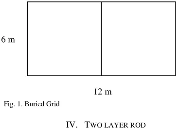
[image:2.612.74.298.192.328.2]

For the grid shown in Fig. 1 the resistance was calculated considering that the resistivity of the upper layer is 3000 Ω_{m, the resistivity of the lower layer is 22}Ω_{m and the} thickness of the upper layer is 0.2 m. The grid was buried to a depth of 0.6 m. Note that the conductors were considered to have an area of 50 mm2 [13]. The obtained value of the resistance using the software program developed was 0.924 Ω_{. This value has an error of 7.6% for the 1}Ω measured value, and a deviation of 5.4% for the 0.987 Ω calculated value [13].

Fig. 1. Buried Grid

IV. TWO LAYER ROD

When considering a rod that crosses through the two layers, calculating the potential at a point that is in a different layer of the point source is required. To calculate the potential in the upper layer, due to a point source in the lower layer, the formula is [11]:

, , _&_%_'&, , , (3)

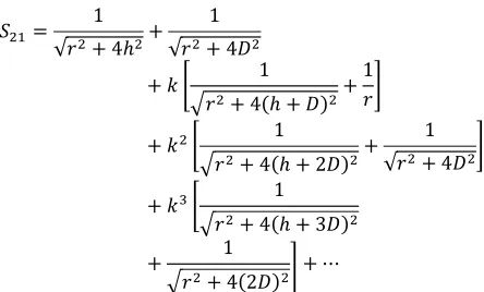
where σi is the conductivity of the ‘i’ layer and S21 is [11]:

, , , , , 2 "

# , ,

2 "

6 m

[image:2.612.318.500.397.530.2]

(3)

For the resistance calculation of a ground rod crossing the two layers the functions V11, V22, and V21 were used. The V12

function was not used because of symmetry in the coefficient matrix [11]. The results for a 2 m length rod and 8 mm radius, buried at ground level, with an upper soil layer of 100 Ω_{m resistivity and a 500}Ω_{m resistivity in the lower} layer are summarized in the third row of Table III. The maximum deviation is 20%. Searching for better results, a discretization in the area close to the discontinuity plane between the two layers was refined, with points separated by 1 mm in the first centimeters above and below the plane z = −D. The remaining points kept the 1 cm discretization. The results in the fifth row show a slight improvement. Finally the entire rod was discretized with source points separated by 1 mm with results presented in the last two rows.

TABLE III

COMPARISON WITH TAGG FORMULA FOR TWO LAYER ROD K=2/3

Parameters/Results 1º SIM 2º SIM 3º SIM

Upper layer thick, D (m) 0.5 1.0 1.5

Resistance (Tagg), (Ω) 134 93.4 72.0

Resistance Matrix Method, ( Ω) 161 103 73.1

Error to Tagg (%) 20 10 1.5

Improved discretization (Ω) 160 102 72.9

Error To Tagg (%) 19 9.2 1.3

1 mm total discretization (Ω) 160 102 69

Error To Tagg (%) 19 9.2 -4.2

Changing the value of the resistivity of the two layers, the values shown in Table IV were obtained.

TABLE IV

COMPARISON WITH TAGG FORMULA FOR TWO LAYER ROD K=-2/3

Resistance (Tagg), (Ω) 60 77 114

Resistance Matrix Method, ( Ω₎ ₅₂ _42.5 _57.6

Error to Tagg (%) -13 -45 -50

Improved discretization (Ω) 51.4 42.3 57.1

Error To Tagg (%) -14 -45 -50

1 mm total discretization (Ω) 51.2 42.2 56.5

Error To Tagg (%) -15 -45 -51

An increase in ground resistance was expected when the upper layer thickness increases, because is more resistive, although this appears not to happen. The errors are unacceptable. The only satisfactory conclusion seems to be that a 1 cm discretization between points is sufficient.

As the examples previously presented validated the V11

and V22 functions, the source of these errors can be

connected with V21, so this function was analyzed in detail.

With this purpose a current point source, PA, in the lower

[image:3.612.316.538.603.737.2]

layer and an upper layer point P sharing the same abscissa and the same ordinate, so the first and second argument of Green function are t=u=0, were considered, Fig. 2.

Fig. 2 Discontinuity points

Both points are equidistant to the discontinuity plane at a distance h, so the difference in quotas between the two points is 2h, while the sum of these quotas is 2D, resulting in the following expression for S21:

, 0,0,

_{|2+ 2 "|} _{|2" 2 "|}

The fractions can only be computed if:

, _"+ and , 1

First condition is easily satisfied. The second condition cannot be satisfied. The point P under consideration is outside the function domain, so the proposed solution is not applicable at this point. If this point is on the ground surface, its potential cannot be calculated.

In the matrix method the equations (1), (2) and (3) must be used at the electrode surface. Since the V21 discontinuity

points are in the axis of the rod, in the upper layer, the calculation is done in the vicinity of a point outside the domain. With a 1 cm discretization, this occurs easily. Usually the surface points are in front off the point source, sharing the same quota. Considering the conductor radius, r, in the difference of ordinates or abscissa, Green function has just only one zero argument, instead of two.

-, 0, ., 0, -, . _/0_'1 (5)

As early mentioned, with the point P(x,y,z) and the point source, equidistant to the discontinuity plane at a distance h, it follows that the difference in quota between the two points is 2h, while the sum of these quotas is 2D. Expanding (3) and grouping the terms with the same power of k, the following expression was obtained:

1

√-₄₊

1 √-_4"

4 1

/-_{4+ "}

1 -5 ₄ 1

/-_{4+ 2"}

1 √-_4"5 #₄ 1

/-_{4+ 3"}

1

(4)

Even for k close to unity, in modulus, which is its maximum value, the terms involving the powers of k can be neglected, since the denominators are too high, because the upper layer thickness, D, is much greater than the rod radius, and the 1/r fraction is dominant, to those involving D.

With this approximation a simplified version of the S21

function was obtained:

8 1

√-₄₊

1 √-_4"

-

Furthermore with k close to unity, in modulus, the second fraction can be neglected, so S21 is simply:

8 1

√-₄₊

-

This simplified equation shows that for k close to unity, the term k/r is dominant and the sign of k defines whenever S21 is positive or negative.

Notice that with the source points separated by 1 cm, the minimum value for h is closer to 1cm so 2h easily becomes greater than the rod radius. If k is negative, S21 is negative

and, using (3), the potential at that conductor surface point will also be negative, which makes no sense since they are assumed to be positive.

To overcome this problem, in the calculation of V21, it

was assumed that the points on the rod surface, in the top layer, could be displaced 0.1 or 0.2 m away from the axis and therefore reduce the influence of k, due to the increasing value of r. With rods with several meters in length, this shifting of surface points is not significant. The results are shown in Table V and Table VI.

For k = 2/3 the results are improved with 0.2 m displacement of the upper electrode surface, since the maximum error is now 15 % instead of the 20 % error of Table III. Notice the values are conservative.

For k = - 2 / 3 the errors were drastically reduced, from 50% to 34% or 32%, but still they remain unacceptable. However, in this case, the results make sense.

TABLE V

COMPARISON WITH TAGG FORMULA FOR TWO LAYER ROD K=2/3

Resistance (Ω) 0.1 m displacement 159 101 74

Error for Tagg (%) 18 8.3 2.2

Resistance 0.2 m displacement, (Ω) 154 99 73

Error for Tagg (%) 15 6 1.4

TABLE VI

COMPARISON WITH TAGG FORMULA FOR TWO LAYER ROD K=-2/3

Resistance 0.1 m displacement, (Ω) 52.6 55.9 77.4

Error to Tagg (%) -12 -28 -34

Resistance 0.2 m displacement, (Ω) 52.4 58.4 77.9

Error to Tagg (%) -13 -24 -32

With increasing thickness of the upper layer, which is more resistive, the electrode resistance also increases. The matrix method results in unacceptable error in the calculation of rods resistance in a two layer soil, when the upper layer is more resistive, a very common case, even displacing the surface points in the upper layer of 0.1 or 0.2 m. When the upper layer is less resistive the method can be used. Using an average value of resistivity in an equivalent homogeneous soil, using the Kindermman and Dwight formulas [10] allows for results below 20%, as shown in Table VII.

The average resistivity is obtained using Kinderman formula [9]:

9: ;_; ;

9 ;

9

where

L1 : Rod lenght in top layer;

L2 : Rod lenght in lower layer

ρ1 : Top layer resistivity;

ρ2 : Down layer resistivity

Using a weighted average value for resistivity in an equivalent homogeneous soil [14], the problem can be solved for k negative.

TABLE VII

COMPARISON WITH TAGG FORMULA USING AN EQUIVALENT

HOMOGENEOUS SOIL

Average Resistivity k=2/3, (Ω/m) 250 167 125

Average Resistivity k=-2/3, (Ω/m) 125 167 250

Dwight formula k=2/3 (Ω) 118 78.4 58.8

Error To Tagg (%) -13 -16 -18

Dwight formula k=-2/3 (Ω₎ _58.7 _78.4 ₁₁₈

Error To Tagg (%) -2 0.1 3

(5)

V. CONCLUSION

The matrix method produces very good results (less than 3 % error) when the electrodes are in a single layer, in a two layer soil. With rods crossing the two layers, if the resistivity of the lower layer is larger, the method gives results with 20 % maximum errors. This error can be reduced by displacing the surface points in the top layer to 0.1 or 0.2 m away from the axis rod.

If the upper layer is the most resistive, a more common case, the method obtains unacceptable results, even displacing the surface points in the upper layer 0.1 or 0.2 m away from the rod axis. The points in the lower layer have images on the upper layer that are discontinuity points of the Sunde solution, not allowing for potential calculations in these points. In the vicinity of those points, for the negative voltage reflexion coefficient, the calculated potential can even be negative. This kind of problem has not been reported in the literature. Although the matrix method is not commonly used, some methods are obtained by integrating the S functions, propagating the discontinuity points.

The use of Kinderman formula for an apparent resistivity in homogeneous soil can overcome the problems for negative reflexion coefficient, exploring the knowledge we have in that soil type.

REFERENCES

[1] Salama, Elsherbiny, Chow. Calculation and interpretation of a grounding grid in two-layer earth with the synthetic-asymptote approach. Electric Power Systems Research 35, 1995.

[2] Berberovic, Haznadar, Stih. Method of moments in analysis of grounding systems. Engineering Analysis with Boundary Elements 27, 2005.

[3] Sharma, De Four, Parametric Analysis of Grounding Systems in Two-Laier Earth using Galerkin’s Moment Method, IEEE 2006.

[4] Colominas, Gomez-Calvino, Navarrina, Casteleiro. A general numeric model for grounding analysis in layered soils. Advances in Engineering Software 33, 2002.

[5] Colominas, Navarrina, Casteleiro, A Numerical Formulation for Grounding Analysis in Stratified Soils, IEEE Transactions on Power Delivery, VOL. 17, NO. 2, April 2002.

[6] Colominas, Aneiros, Navarrina, Casteleiro, A BEM Formulation for Computational Design of Grounding Systems in Stratified Soils, Computational Mechanics: New Trends and Applications, Idelsohn, Onate and Dvorkin (Eds) CIMNE, Barcelona, Spain 1998.

[7] Adriano, Bottauscio, Zucca, Boundary Element Approach for the analysis and design of grounding systems in presence of non-homogeneousness, IEE Proceedings Gener. Transm. Distrb. Vol 150, No. 3, May 2003.

[8] Coa, Comparative Study between IEEE Std.80-2000 anf Finite Elements Method application for Grounding System Analysis, 2006 IEEE.

[9] Ma, Dawalibi, Southey, On the equivalence of uniform and two-layer soils to multilayer soils in the analysis of grounding systems, IEE Proceedings Gener. Transm. Distrb. Vol 143, No. 1, January 1996. [10] Liu, Theethayi, Thottappillil, Gonzalez, Zitnik. An improved model

for soil ionization around grounding systems and its application to stratified soil. Journal of Electrostatics 60, 2004.

[11] Joy, Meliopoulos e Webb, ‘Touch and Step Calculations for Substation Grounding Systems’, approved by the IEEE Substation Committe of the IEEE Power Engineering Society, 1979.

[12] Grounding of Industrial and Commercial Power Systems, IEEE Std 142-2007.

[13] Alonso, Fernandez e Figueras, Modelo para el Analise de Redes de Tierra por Elementos Finitos. Calculo de la Resistência de Tierra. 5º Jornadas Hispano-Lusas de Ingenieria Eléctrica, Salamanca 1997, Actas Tomo I.