Abstract— Over the last few years, gains from financial integration of emerging markets have been a point of debate. Whereas some academics try to demonstrate the benefits of such integration for the country, others show that, because emerging markets behave differently from developed markets, the benefits of financial integration in the latter do not bring the expected results. This paper contributes to the discussion by analyzing the relation between the Colombian stock market’s financial integration and its efficiency levels. To do so, we draw on the multivariate statistical method of principal component analysis to propose a measure of financial integration and then use the covariances of the nonpredictable portion of share returns obtained from the modified CAPM (capital asset pricing model, modified by Fama and French) as a measure of financial efficiency. Our subsequent regression analysis reveals that in the Colombian stock market, financial integration, despite being significantly related to the market’s financial efficiency, does not explain a high portion of its variability, suggesting a need to identify that other variables of greater importance that may affect either the market’s financial integration or its efficiency levels.
Index Terms— Colombian Stock Market, CAPM Three factors model, Financial Efficiency, Financial Integration, Principal Components analysis.
I. INTRODUCTION
I
n the debate over the gains and problems of international financial integration, one side argues that financial market integration between emerging and developed markets generates capital flows that directly increase the economic growth of these markets (Gourinchais and Jeanne, 2003). These scholars also claim that financial integration of any kind is positive because it helps local markets grow larger through access to international markets, which allows companies to exploit economies of scale. More specifically, when companies have strong relations with more developed1 Manuscript received March 26, 2011; revised April 09, 2011. This
work was supported by the Department of Industrial Engineering of the Faculty of Engineering of ―Universidad de Los Andes‖.
Juan David Albán C is an Industrial Engineer with majors in Operations research and Finances of the Engineering Faculty of Los Andes University with a master degree on Operations Research of the Engineering Faculty of Los Andes University. Recently is working on the Reinsurance Market for a local insurance company. (City: Bogotá, Colombia, phone:
57-3165251063; fax: 57-1-6184245; e-mail: [email protected]).
Professor Julio E Villarreal N is the Director of the Economics and
Finance academic area in the Industrial Engineering Department at the Enginnering school at Universidad de los Andes. Bogotá, Colombia. Phone
57 -1 3394949 Ext 2883. E-mail: [email protected]
financial markets, they can reduce their exposure to certain risks via diversification while still benefiting from the greater amount of information available in larger markets (IADB, 2002). That is, when you let international actors have access to a market, its size increases and thus regulatory policies, instead of governing specific market agents, become independent policies. In general, therefore, financial integration helps to prevent ―regulatory arbitrage‖ in local markets as their size increases (Inter-American Development Bank [IADB], 2002).
On the other hand, Gourinchais and Jeanne (2003) find that for some countries (especially emerging nations), the gains from international financial integration are unclear and in some cases even small because of imperfections in capital flows. Some studies even show that the behavior of emerging stock markets does not resemble that of developed stock markets as much as once supposed. Rather, according to Bruner et al. (2003), ―returns in emerging markets are determined more by country factors than by industry factors…[which in turn implies] that emerging markets as an asset class consist largely of assets located in relatively isolated markets, despite progress toward financial liberalization and integration‖ (53).
Accordingly, the benefits of international financial integration in emerging markets like the Colombian stock market remain unclear. That is, although many scholars infer a relation between variables like integration and consumption or integration and growth, they fail, for example, to clearly show the relation between financial efficiency and financial integration for the Colombian equity market. This paper therefore proposes measures of both financial integration and financial efficiency in this market to generate inferences about the relation between these two variables and its significance. If a significant relation exists, the elimination of barriers and restrictions to capital flows has probably reduced information asymmetries inside the market so that stock prices correspond to the information about them known by the market.
The remainder of the article is organized as follows. Section II gives an overview of the Colombian financial market and discusses international financial integration in this context. Section III explains financial efficiency. Section IV then details the measures developed for these variables and their application in the analyses, after which Section V outlines our results and conclusions.
II. FINANCIAL MARKET INTEGRATION
Financial integration can be defined as ―the process through which a country’s financial markets become more closely integrated with those in other countries or with those
Financial Integration and Financial Efficiency:
an Analysis of their Relation in the Colombian
Stock Market
in the rest of the world‖ (IADB, 2002). In general, such integration requires the elimination of barriers that prevent financial institutions in overseas markets (e.g., banks or trading institutions) from supplying services in other countries.
A. Financial integration in stock markets
Although Financial Integration and Financial Liberalization, are highly related, it is important to note that are not the same. As cited in Bekaert and Harvey (2002), liberalizations may not be enough to actually induce foreign investors to take the decision to invest. The market liberalizations are related to break dates of politics such as reducing foreign ownership restrictions, or reducing the different restrictions to capital flows rather than the final decision of an investor to invest, or a company to be part of any specific stock market.
In contrast, Financial Integration depends on how much foreign investors, and foreign companies increase their participation on any specific stock market, and how this situations affect correlations between stocks, discount rates, liquidity, efficiency and Cost of capital, among others.
Financial integration in stock markets can bring major benefits not only to the nation’s financial system as a whole but also to companies that become directly integrated with other markets. Most particularly, financial integration implies that the cost of any asset with a specific risk value in the local market is the same as in global markets. This equivalency makes it impossible for investors to take advantage of the arbitrage opportunities that would result from differences in returns between two equity markets.
If restrictions and legislations are similar worldwide, capital from anywhere can flow into the financial systems of the nations involved and increase their liquidity. As market liquidity levels increase, a reduction is also likely in local market risk factors because of the simultaneous increase on the number of transactions and their volume, helping prices to react to new information. Financial integration is therefore evident both when foreign companies start trading in a local market and when investors from overseas introduce their capital into this market.
III. FINANCIAL MARKET EFFICIENCY
The Financial efficiency is determined by how fast information is incorporated in share prices, and to what extent those prices correspond to the information available about a company on a specific time period. According to Brealey and Myers (1998), a market is efficient if ―information is widely available and in a cheaper way for investors‖ (p. 231) so that all the relevant information about an asset is already included in its price. Hence, since there are no arbitrage opportunities when prices correspond to known information known for an active stock, for a market to be efficient, all transactions must have a net present value of 0. Such market efficiency can be classified into three different levels—weak, semi-strong, and strong (Roberts, 1967).
The primary hypothesis of financial market efficiency theory is that, because prices react only to the information available to the market at any given time, changes in share prices occur randomly. That is, since the information is known throughout the time period, it must be unpredictable
(i.e., were if predictable, it would already have been incorporated into the share price).
Such information is incorporated into share prices through the laws of supply and demand. That is, the moment that the market receives information about an asset, the asset price, which must be higher or lower than the initial price, reflects the new information. When investors learn this new information, they decide whether to sell or buy the asset based on convenience. If many investors want to either sell or buy, the share price will rise or lower until it corresponds with the new market valuation and few investors want to trade it.
Investors, for their part, must be sure that the market in which they invest is efficient, because such efficiency guarantees that any asset price in the market changes according to known information in any given period and not because of any other factor that increases price uncertainty. Because share prices result from the information known about them, investors can develop their own estimations and investment choices if they trust that the information offered by the market is consistent with reality.
IV. MEASURES OF FINANCIAL INTEGRATION AND FINANCIAL
EFFICIENCY
A. Financial integration
To measure the level of the Colombian market’s financial integration with global markets, we compare all local market risk factors with those in the rest of the world. If the Colombian market offers similar compensations as other markets for any specific risk factor, then the market is completely globally integrated; if not, then to identify the final level of integration, we must measure how closely the local market comes to world markets. The measure developed for this analysis is based on Korajczyk’s (1995) proposed use of a portfolio containing 6,500 stocks, including those from emerging markets (like Colombia) and the developed markets of the United States, Japan, Australia, and England.
When markets are not fully integrated, it is possible to recognize certain specific and diversifiable risks using the model rj,t
j,t... ...bj,11,t...bj,kk,tj,t. This equationrepresents the return of a stock j in the period t through the expected return
t j,
and includes all the risks factors with their respective weights in the modelbj,11,t. This model, which should decrease in size as database size increases, also includes the error term
t j,
associated with the unexplainable risks of a specific stock.
First, drawing on the historical information for each asset price in the database between March 31, 1995 and December 31, 2005, we use principal component analysis (PCA) to build portfolios that replicate the different risk factors for global markets. One major strength of this method is that it enables extraction of different factors that are lineally independent of each other, each of which replicates one global risk factor.
This procedure is based on the assumption of the model t
j t k k j t
j t j j
i b b
than
0,t (which corresponds to a risk-free asset). Hence, it reflects the fact that a risk-free asset always has an expected return lower than that of any other asset affected by numerous different risk factors.Set t is the number of time periods for the returns of all shares; n is the number of shares in the database (which for this project corresponds to 4,954 shares for most periods); the n * t matrix
r
n is the excess returns matrix (where excess return is the difference between the return on each share and the return on a risk-free asset for the same period) and refers to the compensation for the specific risks affecting each share. Likewise, b is the n* k matrix of factor loadings for each share; F is the k * t matrix containing the risk premium of each risk factor in the model for each period; and
nis the matrix of returns that cannot be explained by the model and must correspond to diversifiable risks (Ross, as cited in Korajczyk, 1995).
= +
rn bn
F
n (n * t) (n * k) (k * t) (n * k)n
r = Exp. Risk premium
n
b = Excess returns Factor loadings
F
= Div.risksHere, each factor has its own value and importance for the total risk in each period (expected + risk premium). The matrix obtained, F, is multiplied by the factor weights (betas) to obtain the returns on each asset for each period and compare them with the real returns.
We anticipate that the greater the size of the database (number of shares), the smaller the error. Therefore, the difference between the real returns and those obtained experimentally (actor times weights) should mostly correspond to the differential resulting from the barriers, restrictions, and/or regulations of countries that are not fully integrated into world markets. These differences must be reflected in the intercept term from the regression analysis between real returns and risk factors.
To obtain portfolios that reflect the asset returns for each period according to their risk factors, we perform a PCA using an input database that contains the returns of each asset for each period. As the matrix of returns for each risk factor is generated, we carry out a regression analysis in which the dependent variable is the real return for each share and the independent variable is the return for each risk factor in a particular time interval. These calculations produce the betas that explain the relation between each risk factor and the returns for each asset, as well as the corresponding intercepts that reflect the NO-integration level of each share with world markets.
To enable comparisons between each share and combine these into a final market measure, we weight the intercept value for each asset in the Colombian Stock Market Index based on its variance. Because only the distance of each intercept of zero matters, after correcting each asset’s integration measure for heterotedaskicity, we square the measure to eliminate negative values. Finally, we obtain the
average that corresponds to the final NO-Integration measure for the Colombian stock market for each period.
If
i,t represents the intercept of asset i in period t, is the variance of asset i, and n is the number of shares in the Colombian Stock Market Index (IGBC) for each period, then the measure of financial integration for period t is as follows:Database: The database was compiled based on the S&P classification of countries as emerging, frontier, or developed, and the price series for the most important assets of 27 countries were obtained from Bloomberg. The developed countries are Australia (ASX), the United States (Nasdaq, Dow Jones, S&P), England (FTSE), and Japan (Nikkei). The emerging markets are Argentina (Merval), Brazil (Bovespa), Chile (Santiago Stock Exchange), Colombia (IGBC), México (BMV general), Peru (IGBVL), Venezuela (BVC), China (Shangai SE), India (BSE 200), Indonesia (JSE), Korea (KSE), Malaysia (KLSE), the Phillipines (PSE), Sri Lanka (CSE Lanka), Taiwan (TAIEX), Thailand (SET), the Czech Republic (PX 50Index), Hungary (BSE Bux Index), Poland(Warsaw), Egypt (Egyptian Financial Group), and Bahrain (BSE composite). The final database contains information about 24 countries and 27 different indexes representing a total of 4,954 stocks having monthly information between February 28, 1995, and January 31, 2006. This dataset corresponds to 131 observations for each asset (unless values are missing for some periods).
Because the information was already recorded in USD, no transformation of database values was necessary. To obtain only that part of the return that corresponds to the response to each asset’s risk factors, we subtract the return in each period for a risk-free asset – indicated by 20 years of U.S. Treasury Bonds for each sample period (http://research.stlouisfed.org, accessed April 5, 2006) – from the returns in the same period for each of the 4,954 assets.
The PCA and corresponding measure of integration level for the market is always performed for 5-year periods beginning with the March 31, 1995, to March 31, 2000, period and ending with the December 31, 2000, to December 31, 2005, period. The analysis includes 70 time intervals based on information for the 4,954 assets in the sample. That is, because some observations in each period have missing values, the number of components obtained for each period varies from 27 to 32, according to the post-PCA regression analysis between each share on the Colombian stock market and the components obtained for each time period.
B. Efficiency of the Colombian stock market
Market efficiency depends not only on the consistency of the information known about an asset and its corresponding price, but also the time the market takes to introduce any particular information on any specific price. Hence, we estimate efficiency to identify the degree of predictability of future returns on shares in the local market in an attempt to differentiate between their predictable (according to the modified CAPM) and nonpredictable portions. As regards
ni t
i t i t
n
IF
1
2 ,
)
1
(
)
/
the latter, market efficiency would correspond to shares’ ―level of randomness‖ as estimated through the covariance between the return of one period and that of the next. If the nonpredictable portion of returns can be highly predicted by the last period’s returns, the market is not even weakly efficient; however, if the relation between the returns in one period and those in the next is small, then the nonpredictable portion of returns (according to the modified CAPM) is truly random and the market is at least weakly efficient.
To obtain the predictable portion of share returns, we choose a modified CAPM model because, according to Bartholdy and Peare (2004), it gives better results (higher r -squares) than the original CAPM model. Indeed, the modified CAPM is probably the best known model for estimating future prices. In this model, the portion of returns that cannot be explained must correspond to ―surprise‖ and thus random (unpredictable) information known by the market at any moment on a time horizon.
C. Fama and French’s three-factor model
The three-factor model that Fama and French (1992) derived after their in-depth investigation assumes that value and size are two of the most significant factors for explaining portions of asset returns in any one period. More specifically, these factors replicate two kinds of risk – size risk and value risk – which together with market risk explain a higher portion of the asset returns. Nonetheless, as Bartholdy and Peare (2004) point out, the higher variability explained by this model is not sufficient to compensate for the difficulty in obtaining the necessary information to perform it.
The volume factor (size risk): The volume factor, which refers to a size premium, helps to measure the additional return that investors gain in each period by investing in assets with lower capitalizations than other market stocks (Borchert et al., 2003).
The value factor: This factor aims to measure the value premium obtained by investors in companies with a higher book-to-market-ratio(BMR)than the norm for their market. A portfolio is obtained by subtracting the returns of market companies with low BMRs from those of firms with high BMRs. A positive value on the value factor shows that, assuming that markets behave efficiently, value stocks (i.e., assets with a high BMR) perform better than ―growing stocks‖ (those with a low BMR) (Borchert et al., 2003).
The equation that corresponds to the modified CAPM is as follows:
where SMB refers to the return of a large company portfolio minus the return of a small company portfolio. Obtaining this variable requires one portfolio in which 50% of the companies have smaller volume values and another in which 50% of companies have higher volume values. To subtract the lower volume values from the higher volume values for use as an independent variable in the regression to explain asset return in each period, we must first obtain the weighted return for each portfolio in each period.
The procedure used to find the return that corresponds to the value factor for each period is similar to that used for the
SMB. We therefore assess each company’s value by comparing its book value, calculated based on firms’ historical cost or countable value, with its market value, determined in the stock market through its market capitalization (http://www.investopedia.com/ terms/b/booktomarketratio.asp, accessed February 12, 2006). The formulation is as follows:
value market Firm
value book Firm market to
Book
For any specific number of companies (in this case, those in each period of the Colombian Stock Market Index), we obtain the weighted average returns for each of the two types of portfolio (that with 50% higher and that with 50% lower BMR) and then subtract the return of the low BMR portfolio from that of the high BMR portfolio.
After finding the value for each factor used in the modified CAPM, we perform a regression in which each factor is an independent variable and the real returns for each period are the dependent variable. By identifying the weight of each factor, this regression provides specifications by which to calculate the return of each asset for the next period. Finally, we obtain the difference between the real value for each period and that derived using the modified CAPM model.
Because the data begin on March 31, 1995, the first estimated return is that for March 31, 2000 (5 years later). After obtaining the nonpredictable return for a monthly series between March 31, 2000, and December 31, 2005, we can calculate the covariance for the nonexplicable returns of one period and the next for 12 (annual) observation series. Finally, we obtain the values between March 31, 2001 (i.e., the covariance of observations between March 31, 2000, and March 31, 2001) and December 31, 2005 (i.e., the covariance between December 31, 2004, and the December 31, 2005) for each asset in the Colombian Stock Market Index. Taking the estimated covariances for each asset and each period, we weight their values so that the variance for each homogenizes with the final sample (as done for the market integration measure).
Whereas some data sets are close to zero, others have considerably higher values than the greater portion of the assets in the sample, meaning that they would have introduced noise into the final measurement of market efficiency. After weighting the covariance for each period and for each asset by each specific variance (i.e., the variance of each asset), we can derive the market average for each period that corresponds to a final measure of the Colombian stock market’s efficiency level.
Setting C oi,tv as the covariance between returns for each
stock i in period t-1 and in period t for a 12-month horizon,
i
v
as the variance of each stock’s covariances I, and n as the number of stocks in the Colombian Stock Market General Index for period t, we produce a final measure of efficiency:) 1 /( ) (
1
,
t
n
i i
t i
t n
V. RESULTS AND CONCLUSIONS
A. Colombian stock market integration
Our first analysis corresponds to the period between March 31, 1996, and March 31, 2001, and our last to the period between December 31, 2000, and December 31, 2005. As the PCA produced a significantly small number of components (60) having the same explained variance as that from the initial database of 4,954 variables, it turned out to be an excellent tool for replicating risk factors matched to those of the world assets sampled. Therefore, not needing to reduce the data further and given the final analytic purpose of creating risk factors (portfolios), we used these 60 components for the next step in the procedure.
Fig. 1 shows the series obtained as a final measure of financial market integration for the period between March 31, 2001, and December 31, 2005. Nonetheless, the results from this current project should not be compared with those from Korajczyk (1995) because, to obtain the final measure of market integration, that author corrected the intercept error term for each period and each asset, whereas we homogenized the final value of the intercept for both.
Fig. 1. Financial Integration. The graph shows high steady values for the first three years of Financial Integration, and a sharp increase on the Integration levels of the last two years.
As Fig. 1 also shows, the market has a tendency to increase integration with the world as the elimination of barriers and capital restrictions and reductions in investor uncertainty increase the flows of free capital. Thus, the high, steady values in the first part of the graph (2001 until 2003) may be a result of the 1999 financial crisis, which caused capital outflow as speculation increased. The integration level then remains steady until the first half of 2003 when the market began to react more positively to the integration with global markets. We also suspect that the country’s integration levels increased following the economic openness of 1991, an ongoing phenomenon resulting not only from elimination of barriers and restrictions to capital flow but also from the generalized openness of other economic sectors. Such openness brought international banking to the country in an effort to improve banks’ business management of their customers’ accounts.
It is, however, important to note that since the data corresponding to March 31, 2001, really reflects what happened in the market between March 31, 1997, and March 31, 2001 (i.e., they encompass the financial crisis), as the datasets move nearer to the 1999 period, the measure of market integration becomes lower and the levels of market
integration higher. We also note that the creation of the Colombian stock market in 2001 led to increased levels of integration.
The results of figure 1 shows how the Colombian Stock Market has integrated gradually during the time horizon of the analysis, and proves, for the Colombian case, that the Financial Integration of the market does not only depend on the elimination of barriers, but also on many market imperfections such as poor liquidity, poor efficiency, and high potential of market manipulation, to actually integrate.
B. Financial efficiency
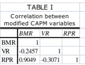
The first aspect analyzed here is the behavior of Fama and French’s three-factor model in the context of the Colombian stock market. Surprisingly, the results reveal a very high correlation between the market factor and the value factor, one that may have caused a multicolinearity problem in the model (see Table 1). Yet despite this high interfactor correlation, the r-square from the modified CAPM model for each period always shows low values that agree with expectations for a model predicting share returns that are inherently unpredictable. Hence, it is not productive to delve further into the possible multicolinearity problem until a model emerges that gives better results than those obtained by Fama and French. We do, however, verify the factor correlations obtained for the model.
Table 1.Correlations between the factors in the modified CAPM model for
the Colombia stock market.
[image:5.595.48.282.327.467.2]As Fig. 2 illustrates, not only are few shares significant at the 10% level, but, surprisingly, the most significant factor is that for value (BMR in the figure). Nonetheless, there is at least one factor (RPR in the figure) that turns out to be more significant than those used in the CAPM.
Fig. 2. Average number of assets that are not significant for each factor and for each period (time intervals begin in the year indicated and finish 5 years
This finding suggests that the Colombian market responds more to value risk than to the other two factors, meaning that this variable from the modified CAPM is better than the 0,0 20000,0 40000,0 60000,0 80000,0 100000,0 120000,0 140000,0 3 1 /0 3 /2 0 00 3 1 /0 6 /2 0 00 3 1 /0 9 /2 0 00 3 1 /1 2 /2 0 00 3 1 /0 3 /2 0 01 3 1 /0 6 /2 0 01 3 1 /0 9 /2 0 01 3 1 /1 2 /2 0 01 3 1 /0 3 /2 0 02 3 1 /0 6 /2 0 02 3 1 /0 9 /2 0 02 3 1 /1 2 /2 0 02 3 1 /0 3 /2 0 03 3 1 /0 6 /2 0 03 3 1 /0 9 /2 0 03 3 1 /1 2 /2 0 03 3 1 /0 3 /2 0 04 3 1 /0 6 /2 0 04 3 1 /0 9 /2 0 04 3 1 /1 2 /2 0 04 3 1 /0 3 /2 0 05 3 1 /0 6 /2 0 05 3 1 /0 9 /2 0 05 3 1 /1 2 /2 0 05 FI Date
BMR VR RPR
BMR 1
VR -0.2457 1
RPR 0.9049 -0.3071 1
TABLE I
Correlation between modified CAPM variables
[image:5.595.384.471.380.446.2] [image:5.595.310.545.553.702.2]market factor used in the basic CAPM to explain asset returns. Nonetheless, weighing the difficulty of obtaining the information needed for the modified CAPM against the improvement in results (from the original CAPM), we conclude that the latter does not compensate for the former. Indeed, as Fig. 3 shows, on average, at a 10% level, no variable is significant for any time period. This observation echoes Bartholdy and Peare’s (2004) finding that, when the three-factor model is applied to a sample of monthly share returns over 5-year periods (taken from Standard & Poor’s), no variables for the 10-year period between 1986 and 1996 show significance at a 5% level.
It is important to note, however, that even though on average, most assets are not significant at the 10% level, certain factors for some assets are significant and help to explain their returns. For example, as Fig. 2 shows, for most of the periods listed in the first part of the graph, approximately half the assets analyzed (between 26 and 30 for the last period) ) are significant for the market factor and value factor, whereas the volume factoris not significant for most of the assets and remains steady during the 2000 to 2006 period.
The significance level of the factors in the model begin lowering in the later periods of the 5-year interval between October 31, 1997, and October 31, 2002. This reduction may be a result of improvements in market efficiency levels subsequent to the 1999 financial crisis. When markets gain efficiency, the significance of factors explaining asset returns lowers (i.e., they have a higher 1-p value), making future prices unpredictable. Hence, the reduction in significance levels in the second part of Fig. 5.4 implies that the market efficiency levels increased after the 1999 financial crisis (between 1999 and 2001), after which they declined gradually (during 2004) before reaching a steady level at the end of the period.
Fig. 3. (1- p value) for each factor and each period (time intervals begin on the period indicated and finish 5 years later). On average, none of the three factors is significant explaining the shares returns.
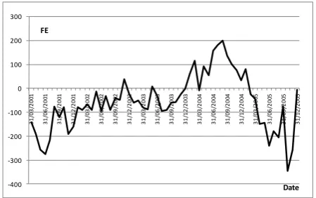
The final assessment of market efficiency levels using the covariance of asset returns suggests that in 2001, 2004, and 2005, the market was less efficient than in 2002 and 2003. Although the inefficient levels of 2001 may again be a consequence of the 1999 financial crisis, the (comparatively) high efficiency values after 2001 might have resulted from the creation of the Colombian stock market, which contributed to an improvement in asset information management and increased controls on speculation, thereby reducing information asymmetries.
Nonetheless, the low levels of efficiency in the last part of the graph might also be related to the behavior of the stock market during the previous year, in which the market showed the highest returns in history. They may thus reflect increased speculation in the market.
Fig. 4. Efficiency level calculated as thecovariance between unexplicable
returns for t and the unexplicable returns for t+1. Covariances are
calculated for a 1-year period. Results of high efficiency on 2002 and 2003 are related to the creation of the Colombian stock market.
C. Relation between financial integration and financial efficiency
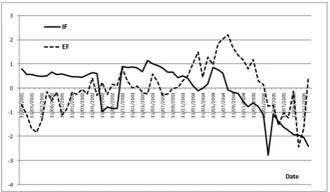
In Fig. 5.5, the measures of the Colombian stock market’s financial integration and financial efficiency between 2001 and 2006, which are calculated on vastly different scales, are standardized for easy comparison. In reality, whereas the financial integration measure has values between 0 and 120,000, the financial efficiency measure has values between -350 and 200. After standardization, however, it becomes clear that the two measures have similar tendencies in particular time periods (see particularly, the last part of Fig. 5.5).
Likewise, the 0.378 correlation coefficient between the two measures indicates that both variables were related during the period of analysis. Moreover, the regression analysis having financial efficiency as the dependent variable and financial integration as the independent variable shows that, at 99% confidence, financial integration is significant enough to explain the variability of the Colombian stock market’s efficiency levels. Nonetheless, according to the 13.36% r-square obtained in the analysis, the percentage of financial efficiency variability explained by financial integration is only 13.36% for the 2001 to 2006 period. These results coincide with those proposed by other scholars (see Sections 1 and 2) who established that, although increased capital flows in any market lead to greater market integration with the world, efficiency levels do not necessarily increase because of problems like imperfections in capital mobility in emerging markets.
[image:6.595.315.540.122.263.2] [image:6.595.57.282.471.615.2]Fig. 5. Comparison between the financial integration measure and the financial efficiency measure (both standardized to facilitate comparison). Smilar trends are observed on the second part of the figure.
Overall, our findings indicate that, although financial integration is significant enough to explain 13.36% of the variability in the Colombian stock market’s financial efficiency, it is not the only variable that affects market efficiency variability. Although these variables are significantly related, an increase on the financial integration level of the market does not increase its efficiency level on the same size.
The Colombian market shows no strong relation between Financial integration and Financial efficiency. Hence, investors and companies from other countries take in to account other factors before deciding to invest on an emerging market. If integration levels increase, there are no real evidences of improvements on efficiency levels through increases in liquidity, reductions of uncertainty and risks diversification as pointed out by some scholars on the first chapter of this article.
Our suggestion for further research in the Colombian stock market is the study of the relation between some aspects like: no common law legislation, integration level of other sectors, cultural and geographical circumstances, specific barriers and taxes, drug dealing money restrictions, exchange rate behavior, country political decisions, (as pointed out by IADB (2002)); and the stock market integration in the Colombian stock market.
REFERENCES
[1] Bartholdy, J., Peare, P., May 2004. Estimation of expected return: CAPM vs. Fama and French. Working paper, Series 176, Centre for Analytical Finance, University of Aarhus.
[2] Bebczuk, R.N., 2003. Asymmetric information in financial markets: Introduction and applications. Cambridge University Press, Cambridge, UK. [3] Bekaert, G., Harvey, C.R., 2000. Foreign
speculators and emerging Equity Markets. The Journal of Finance. Vol LV. No. 2.
[4] Bekaert, G., Harvey, C.R., Lumsdaine, R.L., 2002. Dating the integration of world equity markets. Journal of Financial Economics. 65. Pp 203 – 247. [5] Bekaert, G., Harvey, C.R., Lundblad, C., 2006.
Growth volatility and financial liberalization. Journal of International Money and Finance. 25. Pp 370 – 403.
[6] Borchert, A., Onsz, L. Knijin, J., Pope, G., Smith, A., 2003. Understanding risk and return, the
CAPM, and the Fama-French three-factor model. Tuck School of Business at Dartmouth, City. [7] Brealey, R. A., Myers S. M., 1998. Principios de
finanzas corporativas. Mc Graw Hill series in Finance, Madrid, España.
[8] Bruner, R.F., Conroy, R.M., Li, W., O’Halloran, E.F., Palacios Lleras, M., August 12, 2003. Investing in emerging markets. Association for Investment Management and Research.
[9] Cajueiro, D.O., Gogas, P., Tabak, B.M., December 3, 2008. Does financial liberalization increase the degree of market efficiency? The case of the Athens Stock exchange. International Review of Financial Analysis. 18. Pp 50 – 57.
[10]Cornelis, L.A., Novembr 2, 2004. Measuring the degree of efficiency of financial market efficiency. Kent State University, College of Business Administration and Graduate School of Management. ECONWPA working paper no. 0411003, Accessed December 15, 2005, at http://ideas.repec.org/p/wpa/wuwpfi/0411003.html [11]Gourinchais, P.-O., Jeanne, O., May 2003. The
elusive gains from international financial integration. NBER working paper no. 9684. Available at htttp://www.nber.org/
[12]papersw9684.
[13]Hull. J. C., 2002. Options, Futures and Other Derivatives, Prentice Hall Finance Series, New Jersey.
[14]Inter-American Development Bank, 2002. Financial integration. Retrieved from
http://www.iadb.org/res/publications/pubfiles/pubB -2002E_7384.pdf on December 15, 2005.
[15]Kaminsky, G., Schmukler, S., 1999. On booms and crashes: Stock market cycles and financial liberalization. Latin American and Caribbean economic association LACEA. Retrieved from http://www.lacea.org/meeting2001/SchmuklerK.pd f on December 15, 2005.
[16]Korajczyk, R.A., 1995. A measure of stock market integration for developed and emerging markets. Policy research working paper no. 1482. Accesed January 12 2006.
-4 -3 -2 -1 0 1 2 3
3
1
/0
3
/2
0
01
3
1
/0
5
/2
0
01
3
1
/0
7
/2
0
01
3
1
/0
9
/2
0
01
3
1
/1
1
/2
0
01
3
1
/0
1
/2
0
02
3
1
/0
3
/2
0
02
3
1
/0
5
/2
0
02
3
1
/0
7
/2
0
02
3
1
/0
9
/2
0
02
3
1
/1
1
/2
0
02
3
1
/0
1
/2
0
03
3
1
/0
3
/2
0
03
3
1
/0
5
/2
0
03
3
1
/0
7
/2
0
03
3
1
/0
9
/2
0
03
3
1
/1
1
/2
0
03
3
1
/0
1
/2
0
04
3
1
/0
3
/2
0
04
3
1
/0
5
/2
0
04
3
1
/0
7
/2
0
04
3
1
/0
9
/2
0
04
3
1
/1
1
/2
0
04
3
1
/0
1
/2
0
05
3
1
/0
3
/2
0
05
3
1
/0
5
/2
0
05
3
1
/0
7
/2
0
05
3
1
/0
9
/2
0
05
3
1
/1
1
/2
0
05
IF EF
[image:7.595.51.288.49.187.2]