Clustering and Diversifying Web Search Results with Graph Based Word Sense Induction

Results with Graph-Based Word

Sense Induction

Antonio Di Marco

Roberto Navigli

Sapienza University of Rome

Web search result clustering aims to facilitate information search on the Web. Rather than the results of a query being presented as a flat list, they are grouped on the basis of their similarity and subsequently shown to the user as a list of clusters. Each cluster is intended to represent a different meaning of the input query, thus taking into account the lexical ambiguity (i.e., polysemy) issue. Existing Web clustering methods typically rely on some shallow notion of textual similarity between search result snippets, however. As a result, text snippets with no word in common tend to be clustered separately even if they share the same meaning, whereas snippets with words in common may be grouped together even if they refer to different meanings of the input query.

In this article we present a novel approach to Web search result clustering based on the automatic discovery of word senses from raw text, a task referred to as Word Sense Induction. Key to our approach is to first acquire the various senses (i.e., meanings) of an ambiguous query and then cluster the search results based on their semantic similarity to the word senses induced. Our experiments, conducted on data sets of ambiguous queries, show that our approach outperforms both Web clustering and search engines.

1. Introduction

The Web is by far the largest information archive available worldwide. This vast pool of text contains information of the most wildly disparate kinds, and is potentially capable of satisfying virtually any conceivable user need. Unfortunately, however, in this setting retrieving the precise item of information that is relevant to a given user search can be like looking for a needle in a haystack. State-of-the-art search engines such as Google and Yahoo! generally do a good job at retrieving a small number of relevant results from such an enormous collection of data (i.e., retrieving with high precision, low recall). Such systems today, however, still find themselves up against the lexical ambiguity issue

∗ Dipartimento di Informatica, Sapienza Universit`a di Roma, Via Salaria, 113, 00198 Roma Italy. E-mail:{dimarco,navigli}@di.uniroma1.it.

Submission received: 25 April 2012; revised submission received: 26 July 2012; accepted for publication: 12 September 2012.

(Furnas et al. 1987; Navigli 2009), that is, the linguistic property due to which a single word may convey different meanings.

Recently, the degree of ambiguity of Web queries has been studied using WordNet (Miller et al. 1990; Fellbaum 1998) and Wikipedia1 as sources of ambiguous words.2 It has been estimated that around 4% of Web queries and 16% of the most frequent queries are ambiguous (Sanderson 2008), as also confirmed in later studies (Clough et al. 2009; Song et al. 2009). An example of an ambiguous query isButterfly effect, which could refer to either chaos theory, a film, a band, an album, a novel, or a collection of poetry. Similarly,black spidercould refer to either an arachnid, a car, or a frying pan, and so forth.

Lexical ambiguity is often the consequence of the low number of query words that Web users, on average, tend to type (Kamvar and Baluja 2006). This issue could be solved by expanding the initial query with unequivocal cue words. Interestingly, the average query length is continually growing. The average number of words per query is now estimated around three words per query,3_{a number that is still too low to eradicate} polysemy.

The fact that there may be different informative needs for the same user query has been tackled by diversifying search results, an approach whereby a list of heterogene-nous results is presented, and Web pages that are similar to ones already near the top are prevented from ranking too highly in the list (Agrawal et al. 2009; Swaminathan, Mathew, and Kirovski 2009). Today even commercial search engines are starting to rerank and diversify their results. Unfortunately, recent work suggests that diversity does not yet play a primary role in ranking algorithms (Santamar´ıa, Gonzalo, and Artiles 2010), but it undoubtedly has the potential to do so (Chapelle, Chang, and Liu 2011).

Another mainstream approach to the lexical ambiguity issue is that of Web cluster-ing engines (Carpineto et al. 2009), such as Carrot4 _{and Yippy.}5 _{These systems group} search results by providing a cluster for each specific meaning of the input query. Users can then select the cluster(s) and the pages therein that best answer their information needs. These approaches, however, do not perform any semantic analysis of search results, clustering them solely on the basis of their lexical similarity.

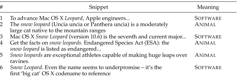
For instance, given the query snow leopard, Google search returns, among others, the snippets reported in Table 1.6In the third column of the table we provide the correct meanings associated with each snippet (i.e., either the operating system or the animal sense). Although snippets 2, 4, and 5 all refer to the same meaning, they have no content word in common apart from our query words. As a result, a traditional Web clustering engine would most likely assign these snippets to different clusters. Moreover, snippet 6 shares words with snippets referring to both query meanings (i.e., snippets 1, 2, and 3 in Table 1), thus making it even harder for Web clustering engines to group search

1http://www.wikipedia.org.

2 Note that we focus here on the ambiguity of queries in terms of their polysemy, rather than on the identification of aspects or subsenses of a given meaning of a query, as was done in recent work on topic identification (Wang, Chakrabarti, and Punera 2009; Xue and Yin 2011; Wu, Madhavan, and Halevy 2011). We discuss this point further in Section 2.6.

3 See Hitwise on 2008–2009 Google data:http://www.hitwise.com/us/press-center/press-releases/ google-searches-apr-09.

4http://search.carrot2.org/stable/search. 5http://search.yippy.com.

Table 1

Some of the top-ranking snippets returned forsnow leopardby Google search.

# Snippet Meaning

1 To advance Mac OS XLeopard, Apple engineers... SOFTWARE

2 Thesnow leopard(Uncia uncia or Panthera uncia) is a moderately

large cat native to the mountain ranges

ANIMAL

3 Mac OS XSnow Leopard(version 10.6) is the seventh and current major... SOFTWARE

4 Get the facts onsnow leopards. Endangered Species Act (ESA): the

snow leopardis listed as endangered...

ANIMAL

5 Snow leopardsare exceptional athletes capable of making huge leaps over

ravines.

ANIMAL

6 Snow Leopard. Even the name seems to underpromise – it’s the

first ‘big cat’ OS X codename to reference

SOFTWARE

results effectively. Finally, none of the top-ranking snippets refers toThe Snow Leopard, a popular 1978 book by Peter Matthiessen.

In this article, we present a novel approach to Web search result clustering that explicitly addresses the language ambiguity issue. Key to our approach is the use of Word Sense Induction (WSI), that is, techniques aimed at automatically discovering the different meanings of a given term (i.e., query). Each sense of the query is represented as a cluster of words co-occurring in raw text with the query. Each search result snippet returned by a Web search engine is then mapped to the most appropriate meaning (i.e., cluster) and the resulting clustering of snippets is returned.

This article provides four main contributions:

r

clustering, which we also exploit to perform a large-scaleend-to-end

experimental comparison of several graph-based WSI algorithms. In fact, the output of WSI (i.e., the automatically discovered senses) is evaluated in terms of both the quality of the corresponding search result clusters and the resulting ability to diversify search results. This is in contrast with most literature in the field of Word Sense Induction, where experiments are mainly performed in vitro (i.e., not in the context of an everyday application; Matsuo et al. 2006; Manandhar et al. 2010).

r

the evaluation measures we implemented in the framework, we complemented our extrinsic experimental evaluation with a qualitative analysis of the automatically induced senses. This study was performed via a manual evaluation carried out by several human annotators.

r

algorithms, namely, SquaT++ and Balanced Maximum Spanning Tree (B-MST) (the former is an enhancement of the original SquaT algorithm [Navigli and Crisafulli 2010], and the latter is a variant of MST [Di Marco and Navigli 2011] that produces more balanced clusters).

r

Table 2

The top five categories returned by the Open Directory Project for the querysnow leopard.

ODP Category # pages

Science: Biology: Flora and Fauna: . . . Felidae: Uncia 6

Kids and Teens: School Time: Science: . . . Leopards: Snow Leopards 4

Science: Environment: Biodiversity: Conservation: Mammals: Felines 3

Kids and Teens: School Time: Science: . . . Animals: Endangered Species 1

Computers: Emulators: Apple: Macintosh: SheepShaver 1

clustering, so as to outperform non-semantic state-of-the-art Web clustering systems. To the best of our knowledge, with the exception of some very preliminary results (V´eronis 2004; Basile, Caputo, and Semeraro 2009), this is the first time that unsupervised text understanding techniques have been shown to considerably boost an Information Retrieval task in a solid evaluation framework.

This article extends previous conference work (Navigli and Crisafulli 2010; Di Marco and Navigli 2011) by performing a novel, in-depth study of the interactions between different corpora and several different WSI algorithms, including novel ones, within the same framework, and, additionally, by providing a comparison with a state-of-the-art search result clustering engine.

The article is structured as follows: in Section 2 we present related work, in Section 3 we illustrate our approach, end-to-end experiments are reported in Section 4, and in vitro experiments are discussed in Section 5. We present a time performance analysis in Section 6, and conclude the paper in Section 7.

2. Related Work

Our work is aimed at addressing the difficulties arising within the different approaches to the issue of lexical ambiguity in Web Information Retrieval. Given the large body of work in this field, in this section we summarize the main research directions on the topic.

2.1 Web Directories

In Web 1.0—mainly based on static Web pages—the solution to clustering search results was that of manually organizing and categorizing Web sites. The resulting repositories are calledWeb directoriesand list Web sites by category and possible subcategories. These categories are sometimes organized as taxonomies (like in the Open Directory Project, ODP7).

Although Web directories are not search engines, information can be searched therein. So, given a query, the returned search results are organized by category. For instance, given the querysnow leopardthe ODP returns the categories shown in Table 2

(the number of matching Web pages is reported in the second column). As can be seen from this example, the Web directory approach has evident limits:

1. It is static, thus it needs manual updates to cover new pages and new meanings (e.g., the book sense ofsnow leopardis not considered in ODP). 2. It covers only a small portion of the Web (e.g., we only have one Web page

categorized with the computing sense ofsnow leopard, cf. the last row of Table 2).

3. It classifies Web pages using coarse categories. This latter feature of Web directories makes it difficult to distinguish between instances of the same kind (e.g., pages about artists with the same surname classified as Arts:Music:Bands and Artists).

Although methods for the automatic classification of Web documents have been proposed (Liu et al. 2005; Xue et al. 2008, inter alia) and some problems have been tackled effectively (Bennett and Nguyen 2009), these approaches are usually supervised and still suffer from reliance on a predefined taxonomy of categories. Finally, it has been reported that directory-based systems are among the most ineffective solutions to Web information retrieval (Bruza, McArthur, and Dennis 2000).

2.2 Semantic Information Retrieval

A second approach to query ambiguity consists of associating explicit semantics (i.e., word senses or concepts) with queries and documents, that is, performingSemantic Information Retrieval (SIR). SIR is performed by indexing and searching concepts rather than terms, that is, by means of Word Sense Disambiguation (WSD; Navigli 2009), thus potentially coping with two linguistic phenomena: expressing a single meaning with different words (synonymy) and using the same word to express various different meanings (polysemy). The main idea is that assigning concepts to words can potentially overcome these two issues, enabling a shift from the lexical to the semantic level to be achieved.

Over the years, various methods for SIR have been proposed (Krovetz and Croft 1992; Voorhees 1993; Mandala, Tokunaga, and Tanaka 1998; Gonzalo, Penas, and Verdejo 1999; Kim, Seo, and Rim 2004; Liu, Yu, and Meng 2005, inter alia). Contrasting results have been reported on the benefits of these techniques, however: It has been shown that WSD has to be very accurate to benefit Information Retrieval (Sanderson 1994)—a result that was later debated (Gonzalo, Penas, and Verdejo 1999; Stokoe, Oakes, and Tait 2003). Also, it has been reported that WSD has to be very precise on minority senses and uncommon terms, rather than on frequent words (Krovetz and Croft 1992; Sanderson 2000).

it is still to be shown that their use for SIR is beneficial. Moreover, these resources do not yet tackle the dynamic evolution of language.

In contrast, our WSI approach to search result clustering automatically discovers both lexicographic and encyclopedic senses of a query (including new ones), thus taking into account all of the mentioned issues.

2.3 Search Result Clustering

A more popular approach to query ambiguity is that of search result clustering. Typ-ically, given a query, the system starts from a flat list of text snippets returned from one or more commonly available search engines and clusters them on the basis of some notion of textual similarity. At the root of the clustering approach lies van Rijsbergen’s cluster hypothesis (van Rijsbergen 1979, page 45): “closely associated documents tend to be relevant to the same requests,” whereas results concerning different meanings of the input query are expected to belong to different clusters.

Approaches to search result clustering can be classified as data-centric or description-centric (Carpineto et al. 2009). The former focus more on the problem of data clustering than on presenting the results to the user. A pioneering example is Scatter/Gather (Cutting et al. 1992), which divides the data set into a small number of clusters and, after the selection of a group, performs clustering again and proceeds iteratively. Developments of this approach have been proposed that improve on cluster quality and retrieval performance (Ke, Sugimoto, and Mostafa 2009). Other data-centric approaches use agglomerative hierarchical clustering (e.g., LASSI [Maarek et al. 2000]), rough sets (Ngo and Nguyen 2005), or exploit link information (Zhang, Hu, and Zhou 2008).

Description-centric approaches are, instead, more focused on the description to produce for each cluster of search results. Among the most popular and successful approaches are those based on suffix trees. Suffix trees are rooted directed trees that contain all the suffixes of a strings. The label of each edge is a non-empty substring of

s and each vertex v is labeled with the concatenation of the edge labels on the path from the root to v. If we view the search result snippets to be clustered as a set of strings (i.e., their bag of words), each vertex of the corresponding suffix tree can be considered as a set of documents that share a phrase (i.e., the label of the vertex itself) and therefore the vertices represent a set of base clustersB=(b1,b2,. . .,bn). The original Suffix Tree Clustering (STC; Zamir et al. 1997; Zamir and Etzioni 1998) algorithm obtains the final clustering by merging the clusters inBwith a high overlap in the documents they contain. A scoring function is defined, based on both the number of documents in the base cluster and the length of the common phrase, with the aim of returning only the topkclusters.

Later developments improved the performance of the STC algorithm using document–document similarity scores in order to overcome the low scalability of the original approach (Branson and Greenberg 2002). Crabtree, Gao, and Andreae (2005) identified an issue in the original scoring function whereby unreasonably high scores tend to be assigned to clusters obtained as a result of the merging of very similar base clusters. To solve this problem, they proposed the Extended Suffix Tree Clustering algorithm (ESTC) with a novel scoring function and a new procedure for selecting the topkclusters to be returned.

S={s1,s2,. . .,s|S|}) in order to choose meaningful labels for the output clusters (Bernardini, Carpineto, and D’Amico 2009; Carpineto, D’Amico, and Bernardini 2011).

Other approaches to description-centric search result clustering in the literature are based on formal concept analysis (Carpineto and Romano 2004), singular value decomposition (Osinski and Weiss 2005), spectral clustering (Cheng et al. 2005), spectral geometry (Liu et al. 2008), link analysis (Gelgi, Davulcu, and Vadrevu 2007), and graph connectivity measures (Di Giacomo et al. 2007). Search result clustering has also been viewed as a supervised salient phrase ranking task (Zeng et al. 2004).

Whereas search result clustering has heretofore been performed without the explicit use of lexical semantics, in our work we show how to exploit search result clustering as the common evaluation framework of both semantic and non-semantic clustering engines.

2.4 Diversification

Rather than clustering the top search results by their similarity, one can aim at reranking them on the basis of criteria that maximize their diversity, so as to present top results which are as different from each other as possible. This technique, calleddiversification of search results, is a recent research topic that, yet again, deals with the query ambiguity issue. To some extent, today’s search engines, such as Google and Yahoo!, apply some diversification technique to their top-ranking results.

One of the first examples of diversification algorithms was based on the use of similarity functions to measure the diversity between documents and between docu-ment and query (Carbonell and Goldstein 1998). Other diversification techniques use conditional probabilities to determine which document is most different from higher-ranking ones (Chen and Karger 2006), or use affinity higher-ranking (Zhang et al. 2005), based on topic variance and coverage.

An algorithm called Essential Pages (Swaminathan, Mathew, and Kirovski 2009) has been proposed that aims to reduce information redundancy and returns Web pages that maximize coverage with respect to the input query. In this approach the Web search results for a queryqare transformed into bags of words containing the terms occurring in the corresponding Web page. Frequency information from raw corpora is then used to find relevant words forq, that is, words which are generally infrequent, but occur often in the results retrieved forq. The coverage score of a search resultris then calculated as a function of the number of terms relevant forqand contained in

r. Another interesting approach reformulates the problem explicitly in terms of how to minimize the risk of dissatisfaction for the average user (Agrawal et al. 2009). A greedy algorithm is proposed that balances between relevance and diversity of the search results. The algorithm is evaluated using generalizations of classical Information Retrieval metrics that are based on statistical considerations and take into account the intentions of the user.

More recently, vector space model representations have been explored to improve diversity in search results (Santamar´ıa, Gonzalo, and Artiles 2010). Web page results are represented as vectors and compared against vector representations of encyclopedic entries available from Wikipedia using cosine similarity. Search results are diversified accordingly.

(2010), who cluster search results by exploiting the links in Web pages in order to identify the subtopics of the returned documents.

2.5 Word Sense Induction

A fifth solution to the query ambiguity issue is Word Sense Induction (WSI), namely, the automatic discovery of word (i.e., query) senses from raw text (see Navigli [2009, 2012] for a survey). WSI allows us to go beyond the surface similarity of Web snippets (which hampers the performance of Web search result clustering) by dynamically acquiring an inventory of senses of the input query. The core idea is to then use these query senses to cluster the Web snippets returned by a traditional search engine.

Very little work on this topic exists: Vector-based WSI was successfully shown to improve bag-of-words ad hoc Information Retrieval (Sch ¨utze and Pedersen 1995) and preliminary studies (Udani et al. 2005; Chen, Za¨ıane, and Goebel 2008) have provided interesting insights into the use of WSI for Web search result clustering. A more recent attempt at automatically identifying query meanings is based on the use of hidden topics (Nguyen et al. 2009). In this approach, however, topics (estimated from a uni-versal data set) are query-independent and thus their number needs to be established beforehand. In contrast, we aim to cluster snippets on the basis of a dynamic and finer-grained notion of sense.

An exploratory study on ten query words has shown that the majority of relevant uses of query words can be identified using graph-based WSI (V´eronis 2004). In the present work we take this preliminary finding to the next level, by studying the impact of several graph-based WSI algorithms on a large scale and by integrating them into a Web search result clustering framework. As a result, we are able not only to perform an end-to-end evaluation of WSI approaches, but also to compare them with traditional search result clustering techniques, which instead lack explicit semantics for the query meanings.

2.6 Aspect Identification

This line of research has some points of contact with WSI, but also important differences:

r

very fine-grained facets of a given query, such as those of rental, pricing, and accidents of a car, in contrast to WSI whose goal is that of inducing different meanings of the given query, such as car as a motor vehicle, railroad car, song, novel, or even primitive in the LISP programming language. In this respect, the two tasks are complementary, because once WSI has discovered the different senses of a query, then one can apply aspect identification to detect subsenses of each meaning.

r

which are not always available in all languages. WSI relies instead on raw text corpora, which can easily be obtained for any language. This difference also holds for custom search engines not working on the Web, which might not have enough statistics from their users, but could instead resort to raw (domain) corpora.

r

query logs and clickthrough data, therefore making research on this topic hard to replicate and evaluate objectively, especially in comparison with other systems.

The framework presented in this article focuses on the ambiguity of queries at the meaning level, leaving the further application of aspect identification techniques to future work, in the hope that the previously mentioned issues of privacy and availability will somehow be mitigated.

3. Semantically Enhanced Search Result Clustering

Web search result clustering is usually performed in three main steps:

1. Given a queryq, a search engine is used to retrieve a list of results

R=(r1,. . .,rn).

2. A clusteringC=(C1,. . .,Cm) of the results inRis obtained by means of a clustering algorithm.

3. The clusters inCare optionally labeled with an appropriate algorithm (e.g., Zamir and Etzioni 1998; Carmel, Roitman, and Zwerdling 2009) for visualization purposes.

First, we preprocess the set R of search results returned by the search engine (Section 3.1). Next, to inject semantics into search result clustering, we propose improving Step 2 by means of a WSI algorithm: Given a queryq, we first dynamically induce, from a text corpus, the set of word senses ofq(Section 3.2); next, we cluster the Web results on the basis of the word senses previously induced (Section 3.3). We show our framework in Figure 1.

3.1 Preprocessing of Web Search Results

Figure 1

The workflow of semantically enhanced Web search result clustering.

each resultriis processed by means of four steps aimed at transforming it into a bag of wordsbi:

1. We obtain the snippetsicorresponding to the resultri.

2. We apply tokenization tosi, thus splitting the string into tokens and setting them to lowercase.

3. We augment the current token set with multi-word expressions obtained by compounding subsequent word tokens up toφwords (a parameter whose tuning is described later in Section 4.1.4). The terms in the resulting token set are lemmatized using WordNet as reference lexicon. We remove tokens that are not in the WordNet lexicon (e.g.,the,esa).

4. We remove the stopwords (e.g.,get,on,be,as) and the target query words (e.g.,snow,leopard,snow leopard) from the token set.

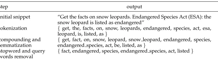
An example of the application of the four steps to a snippet returned for the querysnow leopardis shown in Table 3. As a result of this process, we obtain a list of bags of words

B=(b1,. . .,bn), wherebiis the bag of words of the search resultri.

3.2 Graph-Based Word Sense Induction

The next step is to dynamically discover the senses of the input queryqand provide a representation for them that will later be used for semantically clustering the snippets preprocessed in the previous step. WSI algorithms are unsupervised techniques aimed at automatically identifying the set of senses denoted by a word. These methods induce word senses from text by clustering word occurrences on the basis of the idea that a

Table 3

Processing steps for one of the search results of the querysnow leopard.

step output

initial snippet “Get the facts on snow leopards. Endangered Species Act (ESA): the snow leopard is listed as endangered”

tokenization {get, the, facts, on, snow, leopards, endangered, species, act, esa, leopard, is, listed, as}

compounding and lemmatization

{get, fact, on, snow, leopard, snow leopard, endangered, species, endangered species, act, be, listed, as}

stopword and query words removal

given word—used in a specific sense—tends to co-occur with the same neighboring words (Harris 1954). Several approaches to WSI have been proposed in the literature (see Navigli [2009, 2012] for a survey), ranging from clustering based on context vectors (e.g., Sch ¨utze 1998) and word similarity (e.g., Lin 1998) to probabilistic frameworks (Brody and Lapata 2009), latent semantic models (Van de Cruys and Apidianaki 2011), and co-occurrence graphs (e.g., Widdows and Dorow 2002).

In our work, we chose to focus on approaches based on co-occurrence graphs for two reasons:

i) They have been shown to achieve state-of-the-art performance in standard evaluation tasks (Agirre et al. 2006b; Agirre and Soroa 2007; Korkontzelos and Manandhar 2010).

ii) Other approaches are either based on syntactic dependency statistics (Lin 1998; Van de Cruys and Apidianaki 2011), which are hard to obtain on a large scale for many domains and languages, or based on large matrix computation methods such as context-group discrimination (Sch ¨utze 1998), non-negative matrix factorization (Van de Cruys and Apidianaki 2011) and Clustering by Committee (Lin and Pantel 2002). Instead, in our approach we aim to exploit the relational structure of word co-occurrences with lower requirements (i.e., using just a stopword list, a lemmatizer, and a compounder, cf. Section 3.1), assuming that the semantics of a word are represented by means of a co-occurrence graph whose vertices are co-occurrences and whose edges are co-occurrence relations.

We therefore integrated the following algorithms into our framework:

r

participation ratio of words in graph triangles, that is, complete graphs with three vertices.

r

integrates two graph patterns previously exploited in the literature (Navigli and Crisafulli 2010), namely, squares and triangles, with a novel pattern called diamond.

r

a WSI algorithm based on the calculation of a Maximum Spanning Tree (Di Marco and Navigli 2011) that aims at balancing the number of co-occurrences in each sense cluster.

r

(representing basic meanings) in co-occurrence graphs.

r

partitions the graph vertices by iteratively transferring the mainstream message (i.e., word sense) to neighboring vertices.

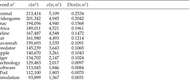
Table 4

Example co-occurrences of wordw=lion.

wordw c(w) c(w,w) Dice(w,w)

animal 213,414 5,109 0.2534

videogame 201,342 4,945 0.2042

mac 194,056 4,940 0.1568

africa 189,011 4,521 0.1961

feline 167,487 4,548 0.1472

cat 161,980 4,493 0.1214

savannah 159,693 3,535 0.1091

predator 145,239 3,643 0.1065

apple 140,670 3,261 0.1043

tiger 134,702 2,147 0.1024

technology 129,483 2,017 0.0097

software 113,045 1,846 0.0084

iPod 112,100 1,803 0.0070

simulation 93,899 1,367 0.0031

3.2.1 Step 1: Graph Construction.Given a target queryq, we build a co-occurrence graph

Gq=(V,E) such that V is the set of words8 co-occurring with q, and E is the set of undirected edges, each denoting a co-occurrence between pairs of words in V. We harvest the statistics for co-occurring wordsVfrom a text corpus (we used two different corpora, see Section 4.1.2), which was previously tokenized and lemmatized.

First, for each word wwe calculate the total numberc(w) of its occurrences and the number of times c(w,w) thatwoccurs together with some word w in the same context (to this end, we use the lemmas corresponding to inflected forms in the text). For instance, in Table 4, assumingw=lion, we show the absolute countc(w) of some words (second column) together with the joint co-occurrence countc(w,w) of wordsw

occurring withw=lionin the same context (third column). Note that the co-occurrences

w may refer to different senses of wordw—for example,africa and savannahrefer to the animal sense oflion, whereastechnologyandsoftwareto the operating system sense. Moreover,wmay be ambiguous itself in the context ofw(e.g.,tigeras either an animal or an operating system).

Second, we calculate the Dice coefficient to determine the strength of co-occurrence between any two wordswandw:9

Dice(w,w)= 2c(w,w ₎

c(w)+c(w). (1)

Table 4 reports the Dice coefficients in the fourth column for the example words. The rationale behind the use of the Dice coefficient, as opposed to, for example, a simple co-occurrence count such asc(w,w), is that dividing by the average of the total

8 Because our application (i.e., Web search result clustering) typically deals with nominal senses, and to avoid overly large graphs, we restrict our vocabulary to nouns only.

counts of the two words drastically decreases the ranking of words that tend to co-occur frequently with many other words (home,page, etc.).

Finally, we use the occurrence and co-occurrence counts just collected to construct the co-occurrence graph Gq=(V,E) for the input query q. The pseudocode of our graph construction procedure is shown in Algorithm 1 and consists of the following steps:

a. Initialization with snippet words(lines 1–2):Initially we setVto contain all the content words from the bags of words obtained from the snippet results of queryq, that is,V:=_jn₌₁bj, wherebjis the bag of words corresponding to the search resultrj∈Ras obtained after the preprocessing step (see Section 3.1). We also setE:=∅, that is, the edge set is initially empty.

b. Adding first-order co-occurrences(lines 3–5):We augmentVwith the highest-ranking words co-occurring with queryqin the selected text corpus, that is, those wordswfor which the following equations are satisfied:

⎧ ⎨ ⎩

c(q,w)

c(q) ≥δ

Dice(q,w)≥δ

(2)

whereδandδare experimentally tuned thresholds (cf. Section 4.1.4). c. Adding second-order co-occurrences(lines 6–11):Optionally, we create an

auxiliary copyV(0)ofV. For each wordw∈V(0)we augmentVwith those wordswwhich are strongly related towin the text corpus. In other words we addwtoVif both Equations (2) are satisfied for the pair of wordsw

andw.

Algorithm 1The graph construction algorithm.

Input: queryq, the bag of words (b1,· · ·,bn) forq

Output: a graphGq=(V,E)

1: V:=n_j=1bj

2: E:=∅

3: for eachwordwin the corpus

4: ifc(q,w)/c(q)≥δandDice(q,w)≥δthen

5: V:=V∪ {w}

6: ifsecond order=true then

7: V(0)_:=V

8: for eachwordw∈V(0)

9: for eachwordwin the corpus

10: ifc(w,w)/c(w)≥δandDice(w,w)≥δthen

11: V:=V∪ {w}

12: for each(w,w)∈V×Vs. t.w=w 13: ifDice(w,w)≥θ then

14: E:=E∪ {{w,w}}

d. Creating the co-occurrence graph(lines 12–15):For each pair of words (w,w)∈V×V, we add the corresponding edge{w,w}toEwith weight

Dice(w,w) if the following condition is satisfied:

Dice(w,w)≥θ (3)

whereθis a confidence threshold for the co-occurrence relation. Note that we use a thresholdδto select which vertices to add to the graphGq (Step [b]) and we use a potentially different thresholdθfor the selection of which edges to add toGq. Finally, we remove fromVall the disconnected vertices (i.e., those with degree 0).

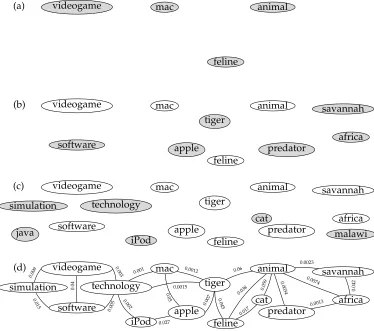
As a result of this algorithm a co-occurrence graph Gq for the query q is pro-duced. Consider again the target word lion and let us assume that the words in Table 4 are the only co-occurrences of lion. In Figure 2 we show the execution of the four steps of our graph construction algorithm for the input query lion, assuming

(a) videogame mac

feline

animal

(b) videogame

software

mac

tiger

apple

animal

feline

savannah

africa predator

(c) videogame

simulation

software

technology

java

mac

tiger

iPod

apple

animal

feline cat

savannah

africa predator _malawi

(d) videogame

simulation

software

technology mac

tiger

iPod

apple

animal

feline cat

savannah

africa predator

0.015 0.009

0.04

0.005 0.003

0.0015

0.002

0.001

0.027

0.05

0.007

0.0012

0.045

0.06

0.038

0.017 0.059

0.0074

0.0034

0.0023

0.0013

0.042

Figure 2

δ=0.38,δ=θ=0.003, andc(lion)=350, 727. First, we initialize the graph with the words in the snippets returned for lion (Figure 2a), next we add the words co-occurring with the query (Figure 2b), then second-order co-occurrences, that is, words co-occurring with those just added to the graph (Figure 2c), and finally we add those edges between word pairs whose Dice value is above a threshold (Figure 2d).

3.2.2 Step 2: Sense Discovery.All the graph-based WSI algorithms that we implemented in our framework are designed to discover the senses of an input term, which in our specific application is the query q. This process of meaning discovery is carried out through the use of the relational and structural information contained in the co-occurrence graph we have just created. In fact, a co-co-occurrence graphGq=(V,E) for a queryqcontains: (i) verticesw∈Vcorresponding to words highly related toq, and (ii) edgese∈Erepresenting co-occurrence relations between vertices (i.e., words) inV. The key idea behind graph-based WSI is to obtain a partition S=(S1,. . .,Sm) of Gq such that each componentSi=(Vi,Ei) contains structurally (i.e., semantically) related vertices (i.e., words). In other words, each vertex setViis intended to contain only words related to a specific sense ofq. As a resultSis thesense inventoryfor the queryqand eachSiis a sense cluster.

We now introduce each graph-based WSI algorithm in detail.

Curvature.The curvature algorithm aims at quantifying how strongly the neighbors of a vertex are related to each other. To measure this degree of correlation, thecurvature

coefficient for a vertexwis calculated as follows:

curv(w)= # triangleswparticipates in

# triangleswcould participate in (4)

where a triangle is a cycle of length 3. The numerator of Equation (4) is trivially calcu-lated as the number of links between neighbors ofw, and the denominator is calculated by counting all the possible pairs of neighbors. According to Equation (4), the curvature coefficient can assume values between 0 and 1. A vertex whose neighbors are highly connected (i.e., with a high value of curvature) is assumed to be part of a component that represents a specific meaning of the target query. Conversely, a vertex with low curvature acts as a connection between different meanings.

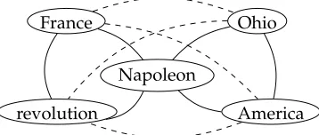
The curvature algorithm is designed to identify the meaning components by means of the removal of all vertices whose curvature is below a certain thresholdσ. For ex-ample, we can attribute two different meanings to the wordNapoleon, namely, a French emperor and an American city. By looking at the graph in Figure 3 we can easily find

Napoleon France

revolution

Ohio

America

Figure 3

thatNapoleonparticipates in two triangles (represented by continuous lines) and it po-tentially could also participate in four additional triangles (i.e., those including dashed lines). It follows that curv(Napoleon)= 2

6 =0.33. The deletion of the vertex Napoleon results in two components (respectively, containing the vertices { France,revolution }

and{Ohio,America}) representing the two mentioned meanings.

SquaT++.The curvature clustering algorithm is based on the hunch that local connec-tivity is correlated with meaning consistency. We take this idea to the next level by proposing a more elaborate local connectivity approach that exploits three different graph patterns, namely: triangles (i.e., cycles of length 3, like in curvature clustering), squares (i.e., cycles of length 4) and diamonds (i.e., graphs with 4 vertices and 5 edges, forming a square with a diagonal), hence the name SquaT++ (Squares, Triangles, and “more”). We determine the strength of the three patterns for a vertex w in the co-occurrence graph as follows:

Tri(w)= # triangleswparticipates in

# triangleswcould participate in (5)

Sqr(w)= # squareswparticipates in

# squareswcould participate in (6)

Dia(w)= # diamondswparticipates in

# diamondswcould participate in (7)

wherewis a vertex. Then we linearly combine the three measures as follows:

SquaT++(w)=α·Tri(w)+β·Sqr(w)+γ·Dia(w) (8)

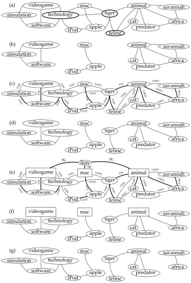
where α+β+γ=1. Similarly to the curvature algorithm, the sense clusters are ob-tained by removing all those vertices whose SquaT++ value is below a thresholdσ. In Figure 4(a) we show in bold the vertices selected for removal, and in Figure 4(b) the sense clusters obtained after removal, namely:{videogame,simulation,software},{iPod,

apple,mac}, and{cat,animal,predator,africa,savannah}.

SquaT++ is a generalization of the curvature algorithm in that: (i) it uses the triangle pattern to calculate curvature, and (ii) it disconnects the graph using the same algorithm as curvature. SquaT++ is a novel algorithm, however, that extends the previously proposed SquaT (Navigli and Crisafulli 2010), based on triangles and squares, by in-troducing a new pattern, namely, the diamond, whose clustering coefficient is linearly combined with the other two. Moreover, in our experiments we tested two versions of SquaT++: the traditional one in which the coefficient is calculated on vertices (like in Equation (8)), and a variant calculated on edges. Our hunch here is that removing low-ranking edges rather than vertices might produce more informative clusters, because no word is removed from the original graph. In what follows, we refer to the vertex version as SquaT++V and to the variant on edges as SquaT++E, and we refer to the general algorithm as SquaT++.

(a) videogame simulation software technology mac tiger iPod apple feline cat animal _savannah africa predator (b) videogame simulation software mac iPod apple animal cat savannah africa predator (c) videogame simulation software technology mac tiger iPod apple animal feline cat savannah africa predator (d) videogame simulation software technology mac tiger iPod apple animal feline cat savannah africa predator (e) lion videogame simulation software technology mac tiger iPod apple animal feline cat savannah africa predator (f) videogame simulation software technology mac tiger iPod apple animal feline cat savannah africa predator (g) videogame simulation software technology mac tiger iPod apple animal feline cat savannah africa predator 0.015 0.009 0.04 0.005 0.003 0.0015 0.002 0.001 0.027 0.05 0.007 0.0012 0.045 0.06 0.038 0.017 0.059 0.0074 0.0034 0.0023 0.0013 0.042 ∞ ∞ ∞ 0.015 0.009 0.04 0.005 0.003 0.0015 0.002 0.001 0.027 0.05 0.007 0.0012 0.045 0.06 0.038 0.017 0.059 0.0074 0.0034 0.0023 0.0013 0.042 Figure 4

the Maximum Spanning Tree (MST) of the co-occurrence graph. Cluster meanings are identified by iteratively removing the edges which represent structurally weak rela-tions, i.e., those with lower weight in the MST. The procedure is as follows:

r

r

qof the graphGq(e.g., the bold edges in Figure 4(c) represent the maximum spanning tree for our initial graph).

r

(2011), iteratively eliminates the minimum-weight edgee∈TGqwhose degree≥2, untilNconnected components (i.e., word clusters) are obtained or there are no more edges to eliminate. The problem with this approach is that it can generate unbalanced clusters (i.e., a few very large clusters and several small clusters); for this reason we developed the B-MST variant which calculates an appropriate cluster mean cardinality10 and removes an edgee∈TGqif its elimination does not lead to connected components with cardinality less than half of the calculated mean value. This additional constraint prevents the creation of very small clusters, while at the same time avoiding artificial equal-size clusters.

Following ourlionexample, and assuming that the value of the only parameter of B-MST (i.e., the maximum numberNof meanings to be identified) is set to 3, we obtain the clusters in Figure 4(d).

HyperLex.Another option for sense discovery is that of HyperLex, which identifies the most interconnected vertices in the graphGq, calledhubs. Each hub acts as the “root” of a specific component ofGqand, correspondingly, a meaning of the target queryq.

First, a listLof the verticeswof the graphGqis created and sorted by their absolute countc(w) in decreasing order. Each vertexw∈Lis then selected as hub if it satisfies the following conditions:

⎧ ⎪ ⎪ ⎪ ⎨ ⎪ ⎪ ⎪ ⎩

degree(w)

maxw_∈Vdegree(w) ≥σ

{w,w}∈EDice(w,w)

degree(w) ≥σ

(9)

that is, the normalized degree of vertex w and the average weight of the edges in-cident on w must be, respectively, above the thresholds σ and σ. Once it has been selected, the hub and all its neighbors are removed fromLso as to avoid neighboring vertices from also being selected as hubs. The hub selection process stops when the next vertex in the sorted list does not satisfy either of the Equations (9) or if the listL

is empty.

As an example, consider the co-occurrence graph in Figure 2(d). A list of the vertices in the graph is created, sorted by c(w), as shown in Table 4. For the purpose of our

example, let us assumeσ=0.5 andσ=0.015. The first hub to be selected isanimal. All its neighbors (tiger,feline,cat,predator,africa, andsavannahin our example) are also removed from the list. The next hub isvideogame(its neighborssimulation,software, and

technologyare also removed from the list). The last hub ismac; after the removal of its neighbor from the list (apple) the last vertex to be examined isiPod, which cannot be selected as hub because it does not satisfy the second condition of Equation (9). The selected hubs are shown as rectangles in Figure 4(e).

Once the hub selection process is complete, the target queryqis added to the set of verticesVof graphGq and each hub is connected toqwith an infinite-weight edge (see vertexlion and its edges added to the graph in Figure 4(e)). Then, a maximum spanning treeTq of the graph is calculated starting from vertexq(see the bold edges in Figure 4(e)). As a result,Tq will include all the infinite-weight edges fromqto its direct descendants, namely, the hubs. Vertexqis then removed from the graph so that each subtree rooted at a hub inTq represents a word sense for the target queryq(see Figure 4(f)). In our example, three clusters are produced:{videogame,simulation,software,

technology},{mac,apple,iPod}, and{animal,feline,tiger,cat,predator,africa,savannah}. Note that, in our example, HyperLex and SquaT++ found the same meanings for the query wordlion(namely, the animal, the operating system, and the videogame), but produced different clusters (e.g., HyperLex assigns the wordtigerto the animal cluster whereas SquaT++ removes it from the graph). Finally, notice that in HyperLex the number of senses is dynamically chosen on the basis of the co-occurrences of qand the algorithm’s thresholds.

An alternative approach to hub selection as performed in HyperLex consists of using the PageRank algorithm to sort the vertices of the co-occurrence graph and choose the best ranking ones as hubs of the target word (Agirre et al. 2006b). Given that the performance of this variant is comparable to that of HyperLex, in this work we focus on the original version of the induction algorithm.

Chinese Whispers.All the previously presented algorithms work in a top–down fashion, that is, they iteratively remove edges or vertices from an initial co-occurrence graph until a number of partitions are obtained. The last algorithm we consider, called Chinese Whispers, works, instead, bottom–up. The pseudocode, shown in Algorithm 2, consists of the following two steps:

1. First, the algorithm assigns a distinct classito each vertexviand creates a clusteringCcontaining the singleton clustersCi(lines 1–4 of the

algorithm).

2. Second, a series of iterations is performed aimed at merging the clusters (lines 5–11). Specifically, at each iteration the algorithm analyzes each vertexvin random order and assigns it to the majority class among those associated with its neighbors. In other words, it assigns each vertexvto the classcthat maximizes the sum of the weights of the edges{u,v}incident onvsuch thatcis the class ofu, according to the following formula:

class(v) :=argmax c

{u,v}∈E(Gq) s.t.class(u)=c

Algorithm 2The Chinese Whispers algorithm.

Input: a graphGq=(V,E) to be clustered

Output: a clusteringCof the vertices inV

1: for eachvi∈V

2: class(vi) :=i

3: Ci:={vi}

4: C:={Ci:i=1,. . .,|V|}

5: repeat

6: C:=C

7: for eachv∈V, randomized order

8: class(v) := argmax

c

{u,v}∈E(Gq)

s.t.class(u)=c

Dice(u,v)

9: for eachidoCi:={v∈V:class(v)=i}

10: C:={Ci:Ci=∅}

11: untilC=C 12: return C

As soon as an iteration produces no change in the clustering (line 11), the algorithm stops and outputs the final clustering (line 12). In contrast to the previous algorithm, Chinese Whispers is parameter-free. Figure 4(g) shows an output example for this algorithm on thelionco-occurrence graph.

3.3 Clustering of Web Search Results

We are now ready to semantically cluster our Web search resultsR, which we previously transformed into bags of wordsB(cf. Section 3.1). To this end we use the automatically discovered senses for our input queryq(cf. Section 3.2). We adopt different measures, each of which calculates the similarity between a bag of words bi∈Band the sense clusters{S1,. . .,Sm}acquired as a result of Word Sense Induction.

Given a result bi, the sense cluster closer to bi will be selected as the most likely meaning ofri. Formally:

Sense(ri)=

⎧ ⎪ ⎨ ⎪ ⎩

argmax

j=1,...,m

sim(bi,Sj) if max

j=1,...,msim(bi,Sj)>0

0 else

(11)

wheresim(bi,Sj) is a generic similarity value betweenbiandSj(0 denotes that no sense is assigned to result ri). As a result of sense assignment for each ri∈R, we obtain a clusteringC=(C1,. . .,Cm) such that:

Cj={ri∈R:Sense(ri)=j} (12)

that is,Cjcontains the search results classified with thej-th sense of queryq.

Word Overlap.It calculates the size of the intersection between the two word sets:

simWO(bi,Sj)=

|bi∩Vj|

|bi|

(13)

whereSj=(Vj,Ej) as defined in Section 3.2.2.

Degree Overlap.It calculates the sum of the degrees in the co-occurrence graph compo-nent ofSjof the snippet’s words inbi:

simDO(bi,Sj)=

w∈bi∩Vjdegree(w,Sj)

|bi| · |Ej|

(14)

wheredegree(w,Sj) is the number of edges incident on win the Sj component of the co-occurrence graph.

Token Overlap. The third measure is similar in spirit to Word Overlap, but takes into account each token occurrence in the snippet bag of wordsbi:

simTO(bi,Sj)=

w∈bi∩Vjc(w,ri)

w∈bic(w,ri)

(15)

wherec(w,ri) is the number of occurrences of the wordwin the resultri.

3.4 Cluster Sorting

As a natural consequence of the different similarity values between snippet results and a given cluster, first, not all the snippets will have the same degree of relevance for the cluster, and second, the produced clusters will show a different “quality” depending on the relevance of the search results therein. We thus sort the clusters in our clustering

C using a similarity-based notion of cluster “quality.” For each clusterCj∈C, we de-termine its similarity with the corresponding meaningSj by calculating the following formula:

avgsim(Cj,Sj)=

ri∈Cjsim(bi,Sj)

|Cj| (16)

The formula determines the average similarity between the bags of words bi of the search resultsriin clusterCjand the corresponding sense clusterSj. The similarity functionsimis the same as that stated in Equation (11) and defined in Section 3.3.

4. In Vivo Experiments: Web Search Result Clustering

We now present two extrinsic experiments aimed at determining the impact of WSI when integrated into Web search result clustering. We first describe our experimental set-up (Section 4.1). Next, we present a first experiment focused on the quality of the output search result clusters (Section 4.2) and a second experiment on the degree of diversification of semantically enhanced versus non-semantic search result clustering algorithms (Section 4.3).

4.1 Experimental Set-up

4.1.1 Lexicon. In all our experiments our lexicon was given by the entire WordNet vocabulary (Miller et al. 1990; Fellbaum 1998) augmented with the set of queries in our test data sets.

4.1.2 Corpora.To calculate the co-occurrence strength between words we need a large corpus to extract co-occurrence counts and calculate the Dice values (cf. Equation (1)). To this end we performed separate experiments on two different corpora and constructed the corresponding co-occurrence databases:

r

collection ofn-grams (n=1,. . ., 5)—namely, windows ofnconsecutive tokens—occurring in one terabyte of Web documents as collected by Google. We consider all the co-occurrences for lemmas which appear in the samen-gram (we applied the WordNet lemmatizer to obtain the canonical form of any word sequence).

r

the.ukdomain and obtaining a large sample of Web pages that were automatically part-of-speech tagged using the TreeTagger tool. For this corpus we considered all the co-occurrences of WordNet lemmas that appear in the same sentence.

We selected these two corpora for their very different natures, namely: Google Web1T is a very large corpus, but with very narrow contexts (5-grams) with a mini-mum occurrence frequency; ukWaC represents a smaller portion of the Web, but with larger contexts. This enabled us to observe the behavior of WSI algorithms when co-occurrences were extracted from different kinds of textual source. In Table 5 we show examples of the contexts available in the two corpora for the same word (i.e.,lion) and the content words that are found to co-occur with it (shown in italics in Table 5).

Table 5

Example of contexts for the wordlionin the Web1T and ukWaC corpora (target word in bold, co-occurring words in italics).

corpus context example

Web1T roarof thelionin

ukWaC Wilson’sZooand itssadlionhad givenwayto thebrave attempttocreateanearly

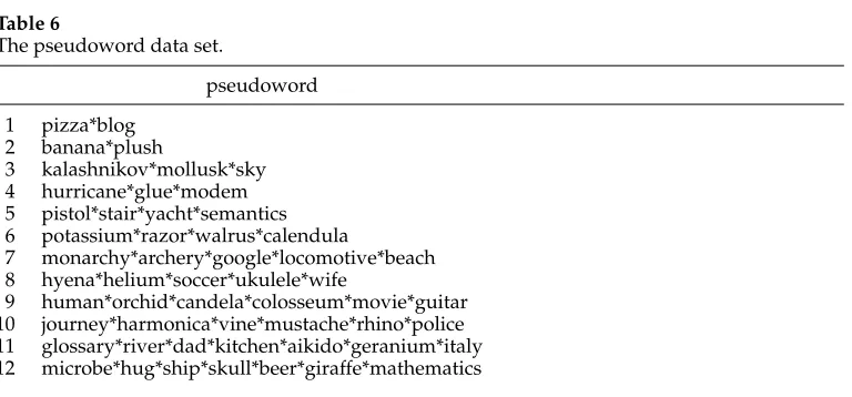
Table 6

The pseudoword data set.

pseudoword

1 pizza*blog

2 banana*plush

3 kalashnikov*mollusk*sky

4 hurricane*glue*modem

5 pistol*stair*yacht*semantics 6 potassium*razor*walrus*calendula

7 monarchy*archery*google*locomotive*beach

8 hyena*helium*soccer*ukulele*wife

9 human*orchid*candela*colosseum*movie*guitar

10 journey*harmonica*vine*mustache*rhino*police 11 glossary*river*dad*kitchen*aikido*geranium*italy 12 microbe*hug*ship*skull*beer*giraffe*mathematics

4.1.3 Tuning Set.Given that our graph construction step and our WSI algorithms have parameters, we created a data set to perform tuning. In order to fix the parameter values independently of our application we created this data set by means of pseudowords (Sch ¨utze 1992; Yarowsky 1993). A pseudoword is an ambiguous artificial word created by concatenating two or more monosemous words. Each monosemous word represents a meaning of the pseudoword. For example, given the words pizzaand blog we can create the pseudoword pizza*blog. The list of pseudowords we used is reported in Table 6.

The powerful property of pseudowords is that they enable the automatic construc-tion of sense-tagged corpora with virtually no effort. In fact, we automatically created our tuning data set as follows:

1. First, we collected the top 100 results retrieved by Yahoo! for each meaning (i.e., monosemous word) of the pseudoword (e.g.,pizzaandblogfor

pizza*blog).

2. We created a set of 100 snippets for the “pseudoword” query (e.g.,

pizza*blog) by selecting snippets from each meaning of the pseudoword in a number that was proportional to their total occurrence count. For instance, ifpizzaandblogoccur, respectively, 73,000 and 27,000 times in the reference corpus (e.g., ukWaC), we selected 73 snippets frompizzaand 27 fromblog. As a result we simulated the distribution of the two senses of the pseudoword within the retrieved snippets.

3. Finally, within each of the 100 snippets, we replaced each monosemous word occurrence (e.g.,pizzaandblog) with the pseudoword itself (i.e.,

pizza*blog). As a result we obtained a set of 100 snippets for each ambiguous pseudoword.

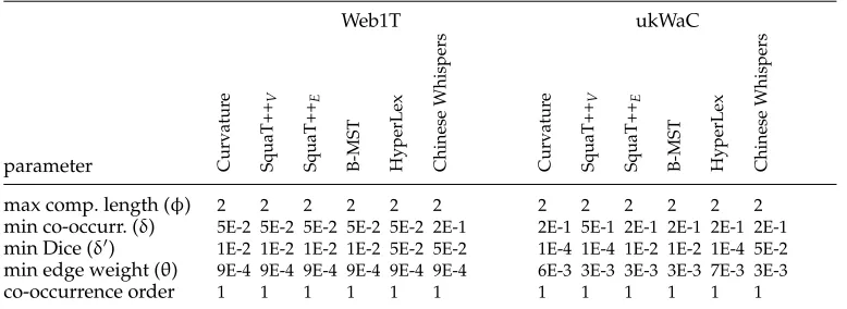
Table 7

The optimal parameter values for graph creation obtained as a result of tuning.

Web1T ukWaC

parameter Curvatur

e

SquaT++

V

SquaT++

E

B-MST HyperLex Chinese

W

hispers

Curvatur

e

SquaT++

V

SquaT++

E

B-MST HyperLex Chinese

W

hispers

max comp. length (φ) 2 2 2 2 2 2 2 2 2 2 2 2

min co-occurr. (δ) 5E-2 5E-2 5E-2 5E-2 5E-2 2E-1 2E-1 5E-1 2E-1 2E-1 2E-1 2E-1

min Dice (δ) 1E-2 1E-2 1E-2 1E-2 5E-2 5E-2 1E-4 1E-4 1E-2 1E-2 1E-4 5E-2

min edge weight (θ) 9E-4 9E-4 9E-4 9E-4 9E-4 9E-4 6E-3 3E-3 3E-3 3E-3 7E-3 3E-3

co-occurrence order 1 1 1 1 1 1 1 1 1 1 1 1

Graph construction. Because all our WSI algorithms draw on the co-occurrence graph, we first tuned the parameters for graph construction for each of the two corpora (cf. Section 3.2.1), namely: the maximum length of the compounds extracted from the corpus (φ), the minimum number of co-occurrences (δ) and minimum Dice value (δ) for vertex addition, and the minimum weight for a graph edge (θ) and vertex addition using first versus second-order co-occurrences. In Table 7 we show the values for these parameters that optimize the performance of each WSI algorithm on the two corpora.11 In all our runs we used the Word Overlap as a similarity measure for Web search result clustering.

We observed that the optimal values for many of the parameters used for graph construction were stable across algorithms, whereas they changed across corpora due to the different scales of the two corpora. Instead, the maximum compound length and the co-occurrence order were fixed for all configurations. For the former we observed no performance increase with longer compound lengths. For the latter we found negligible improvements with second-order co-occurrences, at the cost, however, of increasing the size of the resulting graph exponentially. Given the large number of experiments that would be involved, we decided to avoid this additional workload and use first-order co-occurrences in all our experiments.

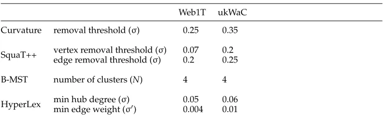
WSI algorithms. Next, for each graph-based WSI algorithm, we kept the given optimal values fixed for building the co-occurrence graphs for the tuning set queries, while varying the parameter values of the WSI algorithm, using Word Overlap as similar-ity measure for Web search result clustering. In Table 8 we show the optimal values for each algorithm when using Web1T (third column) and ukWaC (fourth column) to build the co-occurrence graph. Chinese Whispers is not shown as it is parameter-free (cf. Section 3.2.2). For SquaT++, together with theσthreshold, we also tuned the three coefficient valuesα,β, andγ, that is, we needed to find the best values for the coefficients in Equation (8). The optimal coefficient combinations are shown in Table 9 for SquaT++ on vertices and edges, when using the two corpora for graph construction. The values indicate that all the three graph patterns provide a positive contribution to the algorithm’s performance, with the same coefficients for SquaT++ on vertices and

Table 8

The WSI algorithms’ parameters.

Web1T ukWaC

Curvature removal threshold (σ) 0.25 0.35

SquaT++ vertex removal threshold (σ) 0.07 0.2

edge removal threshold (σ) 0.2 0.25

B-MST number of clusters (N) 4 4

HyperLex min hub degree (σ) 0.05 0.06

min edge weight (σ) 0.004 0.01

Table 9

Optimal values for the three graph patterns used in SquaT++.

Web1T ukWaC

α β γ α β γ

SquaT++V 0.34 0.16 0.50 0.34 0.50 0.16

SquaT++E 0.34 0.16 0.50 0.34 0.50 0.16

edges. Interestingly, we observe that, whereas the contribution of triangles (weighted byα) is the same across corpora, the respective weights of squares (β) and diamonds (γ) are flipped. After inspection we found that the graphs obtained with Web1T are less interconnected than those produced with ukWac. Consequently, diamonds are sparser but more reliable in the Web1T setting, whereas they are much more frequent, and thus noisier, in the ukWaC setting.

4.1.5 Test Sets.We conducted our in vivo experiments on two test sets of ambiguous queries:

r

queries.12_{The sense inventory for the meanings (i.e., subtopics)}13_of queries is given by Wikipedia disambiguation pages. For instance, given thebeaglequery, its disambiguation page in Wikipedia provides the meanings of dog, Mars lander, computer search service, beer brand, and so forth. The top 100 Web results of each query returned by the Yahoo! search engine were tagged with the most appropriate query senses according to Wikipedia (amounting to 4,400 sense-annotated search results). To our knowledge, this is currently the largest data set of ambiguous queries available on-line. In fact, other existing data sets, such as those from the TREC Interactive Tracks, are not focused on distinguishing the subtopics of a query.

12 http://credo.fub.it/ambient.

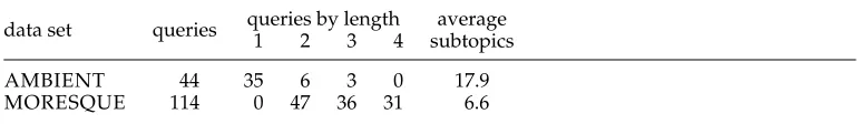
Table 10

Statistics on the AMBIENT and MORESQUE data sets.

data set queries queries by length_{1 2 3 4 subtopics}average

AMBIENT 44 35 6 3 0 17.9

MORESQUE 114 0 47 36 31 6.6

r

developed as an integration of AMBIENT following guidelines provided by its authors.14In fact, our aim was to study the behavior of Web search algorithms on queries of different lengths, ranging from one to four words. The AMBIENT data set, however, is composed in the main of one-word queries. MORESQUE provides dozens of queries of length 2, 3, and 4, together with the top 100 results from Yahoo! for each query annotated precisely as was done in the AMBIENT data set. We decided not to discontinue the use of Yahoo! mainly for homogeneity reasons.

Wikipedia has already been used as a sense inventory by, among others, Bunescu and Pasca (2006), Mihalcea (2007), and Gabrilovich and Markovitch (2009). Santamar´ıa, Gonzalo, and Artiles (2010) have investigated in depth the benefit of using Wikipedia as the sense inventory for diversifying search results, showing that Wikipedia offers much more sense coverage for search results than other resources such as WordNet.

We report the statistics on the composition of the two data sets in Table 10. Given that the snippets could possibly be annotated with more than one Wikipedia subtopic, we also determined the average number of subtopics per snippet. This amounted to 1.01 for AMBIENT and 1.04 for MORESQUE for snippets with at least one subtopic annotation. We can thus conclude that multiple subtopic annotations are infrequent. Finally, we analyzed how the different subtopics are distributed over the snippet results for each query. To do this we calculated the standard deviation of the subtopic popula-tion for each individual query, which we show in Figure 5. We observed a considerable difference in the standard deviations of shorter and longer queries (e.g., between those from the AMBIENT data set [from 1 to 44 in the figure] and the MORESQUE data set [from 45 to 158]). We further calculated the average standard deviation over the two data sets’ queries, obtaining 6.5 for AMBIENT and 13.1 for MORESQUE. Therefore we anticipate that the longer the query length, the more unbalanced will be the distribution of its subtopics over the top-ranking results.

In line with previous experiments on search result clustering, our data set does not contain monosemous queries for two reasons: (i) we are interested in queries with multiple meanings, and (ii) monosemous queries would increase the performance of our experiments because no diversification would be needed for them.

4.1.6 Systems.We performed a comparison of our semantically enhanced search result clustering systems with nonsemantic ones.

0 10 20 30 40 50

0 20 40 60 80 100 120 140 160

std dev

query ID

Figure 5

Standard deviations for the subtopic population of the AMBIENT queries (1–44) and the MORESQUE queries (45–158).

Semantically enhanced systems.We integrated our graph-based WSI algorithms (Curva-ture, SquaT++, B-MST, HyperLex, and Chinese Whispers; cf. Section 3.2) into our search result clustering framework. We tested each algorithm when combined with any of the snippet-to-sense similarity measures introduced in Section 3.3.

Nonsemantic systems.We compared our semantically enhanced systems with four Web clustering engines, namely:

r

in the Carrot open-source framework15that clusters the most frequent phrases extracted using suffix arrays.

r

search clustering approach based on suffix trees.

r

Web clustering engine built on top of STC with part-of-speech pruning and dynamic selection of the cut-off level of the clustering dendrogram.

r

For Lingo and STC we used the Carrot implementation which we integrated into our framework. Conversely, for Yippy we used the on-line output provided by the Web search engine.