Alessandro Moschitti
∗ University of TrentoDaniele Pighin
∗∗ University of TrentoRoberto Basili
†University of Rome “Tor Vergata”
The availability of large scale data sets of manually annotated predicate–argument struc-tures has recently favored the use of machine learning approaches to the design of automated semantic role labeling (SRL) systems. The main research in this area relates to the design choices for feature representation and for effective decompositions of the task in different learning models. Regarding the former choice, structural properties of full syntactic parses are largely employed as they represent ways to encode different principles suggested by the linking theory between syntax and semantics. The latter choice relates to several learning schemes over global views of the parses. For example, re-ranking stages operating over alternative predicate–argument sequences of the same sentence have shown to be very effective.
In this article, we propose several kernel functions to model parse tree properties in kernel-based machines, for example, perceptrons or support vector machines. In particular, we define different kinds of tree kernels as general approaches to feature engineering in SRL. Moreover, we extensively experiment with such kernels to investigate their contribution to individual stages of an SRL architecture both in isolation and in combination with other traditional manually coded features. The results for boundary recognition, classification, and re-ranking stages provide systematic evidence about the significant impact of tree kernels on the overall accuracy, especially when the amount of training data is small. As a conclusive result, tree kernels allow for a general and easily portable feature engineering method which is applicable to a large family of natural language processing tasks.
1. Introduction
Much attention has recently been devoted to the design of systems for the automatic labeling of semantic roles (SRL) as defined in two important projects: FrameNet (Baker, Fillmore, and Lowe 1998), based on frame semantics, and PropBank (Palmer, Gildea,
∗Department of Information Engineering and Computer Science, Via Sommarive, 14 I-38050 Povo (TN). E-mail: [email protected].
∗∗Fondazione Bruno Kessler, Center for Scientific and Technological Research, Department of Information Engineering and Computer Science, Via Sommarive, 18 I-38050 Povo (TN). E-mail: [email protected].
†Department of Computer Science, Systems and Production, Via del Politecnico, 1 I-00133 RM. E-mail: [email protected].
and Kingsbury 2005), inspired by Levin’s verb classes. To annotate natural language sentences, such systems generally require (1) the detection of the target word em-bodying the predicate and (2) the detection and classification of the word sequences constituting the predicate’s arguments.
Previous work has shown that these steps can be carried out by applying machine learning techniques (Carreras and M `arquez 2004, 2005; Litkowski 2004), for which the most important features encoding predicate–argument relations are derived from (shal-low or deep) syntactic information. The outcome of this research brings wide empirical evidence in favor of the linking theories between semantics and syntax, for example, Jackendoff (1990). Nevertheless, as no such theory provides a sound and complete treatment, the choice and design of syntactic features to represent semantic structures requires remarkable research effort and intuition.
For example, earlier studies on feature design for semantic role labeling were car-ried out by Gildea and Jurafsky (2002) and Thompson, Levy, and Manning (2003). Since then, researchers have proposed several syntactic feature sets, where the more recent sets slightly enhanced the older ones.
A careful analysis of such features reveals that most of them are syntactic tree fragments of training sentences, thus a viable way to alleviate the feature design com-plexity is the adoption of syntactic tree kernels (Collins and Duffy 2002). For example, in Moschitti (2004), the predicate–argument relation is represented by means of the min-imal subtree that includes both of them. The similarity between two instances is eval-uated by a tree kernel function in terms of common substructures. Such an approach is in line with current research on kernels for natural language learning, for example, syntactic parsing re-ranking (Collins and Duffy 2002), relation extraction (Zelenko, Aone, and Richardella 2003), and named entity recognition (Cumby and Roth 2003; Culotta and Sorensen 2004).
Furthermore, recent work (Haghighi, Toutanova, and Manning 2005; Punyakanok et al. 2005) has shown that, to achieve high labeling accuracy, joint inference should be applied on the whole predicate–argument structure. For this purpose, we need to extract features from the sentence syntactic parse tree that encodes the relationships governing complex semantic structures. This task is rather difficult because we do not exactly know which syntactic clues effectively capture the relation between the predicate and its arguments. For example, to detect the interesting context, the modeling of syntax-/semantics-based features should take into account linguistic aspects like ancestor nodes or semantic dependencies (Toutanova, Markova, and Manning 2004). In this scenario, the automatic feature generation/selection carried out by tree kernels can provide useful insights into the underlying linguistic phenomena. Other advantages coming from the use of tree kernels are the following.
First, we can implement them very quickly as the feature extractor module only requires the writing of a general procedure for subtree extraction. In contrast, traditional SRL systems use more than thirty features (e. g., Pradhan, Hacioglu, Krugler et al. 2005), each of which requires the writing of a dedicated procedure.
Second, their combination with traditional attribute–value models produces more accurate systems, also when using the same machine learning algorithm in the combi-nation, because the feature spaces are very different.
Third, we can carry out feature engineering using kernel combinations and marking strategies (Moschitti et al. 2005a; Moschitti, Pighin, and Basili 2006). This allows us to boost the SRL accuracy in a relatively simple way.
better and produces a more accurate classifier, especially when the amount of training data is scarce.
Finally, once the learning algorithm using tree kernels has converged, we can iden-tify the most important structured features of the generated model. One approach for such a reverse engineering process relies on the computation of the explicit feature space, at least for the highest-weighted features (Kudo and Matsumoto 2003). Once the most relevant fragments are available, they can be used to design novel effective attribute–value features (which in turn can be used to design more efficient classifiers, e. g., with linear kernels) and inspire new linguistic theories.
These points suggest that tree kernels should always be applied, at least for an initial study of the problem. Unfortunately, they suffer from two main limitations: (a) poor impact on boundary detection as, in this task, correct and incorrect arguments may share a large portion of the encoding trees (Moschitti 2004); and (b) more expensive running time and limited contribution to the overall accuracy if compared with manu-ally derived features (Cumby and Roth 2003). Point (a) has been addressed by Moschitti, Pighin, and Basili (2006) by showing that a strategy of marking relevant parse-tree nodes makes correct and incorrect subtrees for boundary detection quite different. Point (b) can be tackled by studying approaches to kernel engineering that allow for the design of efficient and effective kernels.
In this article, we provide a comprehensive study of the use of tree kernels for se-mantic role labeling. For this purpose, we define tree kernels based on the composition of two different feature functions:canonical mappings, which map sentence-parse trees in tree structures encoding semantic information, and feature extraction functions, which encode these trees in the actual feature space. The latter functions explodethe canonical trees into all their substructures and, in the literature, are usually referred to as
tree kernels. For instance, in Collins and Duffy (2002), Vishwanathan and Smola (2002), and Moschitti (2006a) different tree kernels extract different types of tree fragments.
Given the heuristic nature of canonical mappings, we studied their properties by experimenting with them within support vector machines and with the data set provided by CoNLL shared tasks (Carreras and M `arquez 2005). The results show that carefully engineered tree kernels always boost the accuracy of the basic systems. Most importantly, in complex tasks such as the re-ranking of semantic role annotations, they provide an easy way to engineer new features which enhance the state-of-the-art in SRL. In the remainder of this article, Section 2 presents traditional architectures for SRL and the typical features proposed in literature. Tree kernels are formally introduced in Section 3, and Section 4 describes our modular architecture employing support vector machines along with manually designed features, tree kernels (feature extraction functions), and their combinations. Section 5 presents our structured features (canonical mappings) inducing different kernels that we used for different SRL subtasks. The extensive experimental results obtained on the boundary recognition, role classification, and re-ranking stages are presented in Section 6. Finally, Section 7 summarizes the conclusions.
2. Automatic Shallow Semantic Parsing
lack of a sound and complete linguistic or cognitive theory about the links between syntax and semantics does not allow an informed, deductive approach to the problem. Nevertheless, the large amount of available lexical and syntactic information favors the application of inductive approaches to the SRL task, which indeed is generally treated as a combination of statistical classification problems.
The next sections define the SRL task more precisely and summarize the most relevant work carried out to address these two problems.
2.1 Problem Definition
The most well-known shallow semantic theories are studied in two different projects: PropBank (Palmer, Gildea, and Kingsbury 2005) and FrameNet (Baker, Fillmore, and Lowe 1998). The former is based on a linguistic model inspired by Levin’s verb classes (Levin 1993), focusing on the argument structure of verbs and on the alternation pat-terns that describe movements of verbal arguments within a predicate structure. The latter refers to the application of frame semantics (Fillmore 1968) in the annotation of predicate–argument structures based on frame elements (semantic roles). These theories have been investigated in two CoNLL shared tasks (Carreras and M `arquez 2004, 2005) and a Senseval-3 evaluation (Litkowski 2004), respectively.
Given a sentence and a predicate word, an SRL system outputs an annotation of the sentence in which the sequences of words that make up the arguments of the predicate are properly labeled, for example:
[Arg0He]got[Arg1his money] [C-Vback]1
in response to the input He got his money back. This processing requires that: (1) the predicates within the sentence are identified and (2) the word sequences that span the boundaries of each predicate argument are delimited and assigned the proper role label. The first sub-task can be performed either using statistical methods or hand-crafted lexical and syntactic rules. In the case of verbal predicates, it is quite easy to write simple rules matching regular expressions built on POStags. The second task is more complex and is generally viewed as a combination of statistical classification problems: The learning algorithms are trained to recognize the extension of predicate arguments and the semantic role they play.
2.2 Models for Semantic Role Labeling
An SRL model and the resulting architecture are largely influenced by the kind of data available for the task. As an example, a model relying on a shallow syntactic parser would assign roles to chunks, whereas with a full syntactic parse of the sentence it would be straightforward to establish a correspondence between nodes of the parse tree and semantic roles. We focused on the latter as it has been shown to be more accurate by the CoNLL 2005 shared task results.
According to the deep syntactic formulation, the classifying instances are pairs of parse-tree nodes which dominate the exact span of the predicate and the target argument. Such pairs are usually represented in terms of attribute–value vectors, where
the attributes describe properties of predicates, arguments, and the way they are related. There is large agreement on an effective set of linguistic features (Gildea and Jurafsky 2002; Pradhan, Hacioglu, Krugler, et al. 2005) that have been employed in the vast majority of SRL systems. The most relevant features are summarized in Table 1.
Once the representation for the predicate–argument pairs is available, a multi-classifier is used to recognize the correct node pairs, namely, nodes associated with correct arguments (given a predicate), and assign them a label (which is the label of the argument). This can be achieved by training a multi-classifier on n+1 classes, where the first nclasses correspond to the different roles and the (n+1)th is aNARG (non-argument) class to which non-argument nodes are assigned.
A more efficient solution consists in dividing the labeling process into two steps: boundary detection and argument classification. ABoundary Classifier(BC) is a binary classifier that recognizes the tree nodes that exactly cover a predicate argument, that is, that dominate all and only the words that belong to target arguments. Then, such nodes are classified by a Role Multi-classifier(RM) that assigns to each example the most appropriate label. This two-step approach (Gildea and Jurafsky 2002) has the advantage of only applying BC on all parse-tree nodes. RM can ignore non-boundary nodes, resulting in a much faster classification. Other approaches have extended this solution and suggested other multi-stage classification models (e. g., Moschitti et al. 2005b in which a four-step hierarchical SRL architecture is described).
[image:5.486.57.437.407.670.2]After node labeling has been carried out, it is possible that the output of the argu-ment classifier does not result in a consistent annotation, as the labeling scheme may not be compatible with the underlying linguistic model. As an example, PropBank-style annotations do not allow arguments to be nested. This happens when two or more
Table 1
Standard linguistic features employed by most SRL systems.
Feature Name Description
Predicate Lemmatization of the predicate word
Path Syntactic path linking the predicate and an argument,
e. g., NN↑NP↑VP↓VBX
Partial path Pathfeature limited to the branching of the argument No-direction path LikePath, but without traversal directions
Phrase type Syntactic type of the argument node
Position Relative position of the argument with respect to the predicate Voice Voice of the predicate, i. e., active or passive
Head word Syntactic head of the argument phrase
Verb subcategorization Production rule expanding the predicate parent node Named entities Classes of named entities that appear in the argument node Head word POSPOStag of the argument node head word (less sparse than
Head word)
Verb clustering Type of verb→direct object relation
Governing Category Whether the candidate argument is the verb subject or object Syntactic Frame Position of the NPs surrounding the predicate
Verb sense Sense information for polysemous verbs
overlapping tree nodes, namely, one dominating the other, are classified as positive boundaries.
The simplest solution relies on the application of heuristics that take into account the whole predicate–argument structure to remove the incorrect labels (e. g., Moschitti et al. 2005a; Tjong Kim Sang et al. 2005). A much more complex solution consists in the application of some joint inference model to the whole predicate–argument structure, as in Pradhan et al. (2004). As an example, Haghighi, Toutanova, and Manning (2005) associate a posterior probability with each argument node role assignment, estimate the likelihood of the alternative labeling schemes, and employ a re-ranking mechanism to select the best annotation.
Additionally, the most accurate systems participating in CoNLL 2005 shared task (Pradhan, Hacioglu, Ward et al. 2005; Punyakanok et al. 2005) use different syntactic views of the same input sentence. This allows the SRL system to recover from syntactic parser errors; for example, a prepositional phrase specifying the direct object of the predicate would be attached to the verb instead of the argument. This kind of error prevents some arguments of the proposition from being recognized, as: (1) there may not be a node of the parse tree dominating (all and only) the words of the correct se-quence; (2) a badly attached tree node may invalidate other argument nodes, generating unexpected overlapping situations.
The manual design of features which capture important properties of complete predicate–argument structures (also coming from different syntactic views) is quite complex. Tree kernels are a valid alternative to manual design as the next section points out.
3. Tree Kernels
Tree kernels have been applied to reduce the feature design effort in the context of several natural language tasks, for example, syntactic parsing re-ranking (Collins and Duffy 2002), relation extraction (Zelenko, Aone, and Richardella 2003), named entity recognition (Cumby and Roth 2003; Culotta and Sorensen 2004), and semantic role labeling (Moschitti 2004).
On the one hand, these studies show that the kernel ability to generate large feature sets is useful to quickly model new and not well understood linguistic phenomena in learning machines. On the other hand, they show that sometimes it is possible to manually design features for linear kernels that produce higher accuracy and faster computation time. One of the most important causes of such mixed behavior is the inappropriate choice of kernel functions. For example, in Moschitti, Pighin, and Basili (2006) and Moschitti (2006a), several kernels have been designed and shown to produce different impacts on the training algorithms.
In the next sections, we briefly introduce the kernel trick and describe thesubtree
(ST) kernel devised in Vishwanathan and Smola (2002), the subset tree (SST) kernel defined in Collins and Duffy (2002), and the partial tree (PT) kernel proposed in Moschitti (2006a).
3.1 Kernel Trick
space over the real numbers, namely, n. The learning algorithm uses space metrics over vectors, for example, the scalar product, to learn an abstract representation of all instances belonging to the target class.
For example, support vector machines (SVMs) are linear classifiers which learn a hyperplanef(x)=w×x+b=0, separating positive from negative examples.xis the feature vector representation of a classifying object o, whereas w∈ n and b∈ are parameters learned from the data by applying theStructural Risk Minimization principle (Vapnik 1998). The objectois mapped toxvia a feature functionφ:O→ n,Obeing the set of the objects that we want to classify.ois categorized in the target class only if f(x)≥0.
The kernel trick allows us to rewrite the decision hyperplane as:
f(x)= i=1..l
yiαixi
·x+b= i=1..l
yiαixi·x+b=
i=1..l
yiαiφ(oi)·φ(o)+b=0
whereyiis equal to 1 for positive examples and−1 for negative examples,αi∈ with αi≥0,oi∀i∈ {1,..,l}are the training instances and the productK(oi,o)=φ(oi)·φ(o)
is the kernel function associated with the mappingφ.
Note that we do not need to apply the mapping φ; we can use K(oi,o) directly.
This allows us, under Mercer’s conditions (Shawe-Taylor and Cristianini 2004), to define abstract kernel functions which generate implicit feature spaces. A traditional example is given by the polynomial kernel:Kp(o1,o2)=(c+x1·x2)d, wherecis a constant andd is the degree of the polynomial. This kernel generates the space of all conjunctions of feature groups up todelements.
Additionally, we can carry out two interesting operations:
r
kernel combinations, for example,K1+K2orK1×K2r
feature mapping compositions, for example,K(o1,o2)=φ(o1)·φ(o2)=φB(φA(o1))·φB(φA(o2))
Kernel combinations are very useful for integrating the knowledge provided by the manually defined features with the knowledge automatically obtained with structural kernels; feature mapping compositions are useful methods to describe diverse kernel classes (see Section 5). In this perspective, we propose to split the mappingφby defining our tree kernel as follows:
r
Canonical Mapping,φM(), in which a linguistic object (e. g., a syntactic parse tree) is transformed into a more meaningful structure (e. g., the subtree corresponding to a verb subcategorization frame).r
Feature Extraction,φS(), which maps the canonical structure in all itsfragments according to different fragment spacesS(e. g., ST, SST, and PT).
For example, given the kernel KST=φST(o1)·φST(o2), we can apply a canonical mapping φM(), obtaining KSTM =φST(φM(o1))·φST(φM(o2))=
φST◦φM(o1)·
φST◦ φM(o2), which is a noticeably different kernel, which is induced by the mapping
In the remainder of this section we start the description of our engineered kernels by defining three different feature extraction mappings based on three different kernel spaces (i. e., ST, SST, and PT).
3.2 Tree Kernel Spaces
The kernels that we consider represent trees in terms of their substructures (fragments). The kernel function detects if a tree subpart (common to both trees) belongs to the fea-ture space that we intend to generate. For this purpose, the desired fragments need to be described. We consider three main characterizations: the subtrees (STs) (Vishwanathan and Smola 2002), the subset trees (SSTs) or all subtrees (Collins and Duffy 2002), and the partial trees (PTs) (Moschitti 2006a).
As we consider syntactic parse trees, each node with its children is associated with a grammar production rule, where the symbol on the left-hand side corresponds to the parent and the symbols on the right-hand side are associated with the children. The terminal symbols of the grammar are always associated with tree leaves.
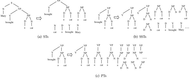
A subtree(ST) is defined as a tree rooted in any non-terminal node along with all its descendants. For example, Figure 1a shows the parse tree of the sentenceMary brought a cattogether with its six STs. Asubset tree(SST) is a more general structure because its leaves can be non-terminal symbols. For example, Figure 1(b) shows ten SSTs (out of 17) of the subtree in Figure 1a rooted inVP. SSTs satisfy the constraint that grammatical rules cannot be broken. For example, [VP [V NP]]is an SST which has two non-terminal symbols, V and NP, as leaves. On the contrary, [VP [V]] is not an SST as it violates the production VP→V NP. If we relax the constraint over the SSTs, we obtain a more general form of substructures that we callpartial trees(PTs). These can be generated by the application of partial production rules of the grammar; consequently [VP [V]]and[VP [NP]]are valid PTs. It is worth noting that PTs consider the position of the children as, for example,[A [B][C][D]]and [A [D][C][B]]only share single children, i.e.,[A [B]],[A [C]], and[A [D]].
[image:8.486.48.435.474.635.2]Figure 1c shows that the number of PTs derived from the same tree as before is still higher (i. e., 30 PTs). These numbers provide an intuitive quantification of the different degrees of information encoded by each representation.
Figure 1
3.3 Feature Extraction Functions
The main idea underlying tree kernels is to compute the number of common substruc-tures between two trees T1 andT2 without explicitly considering the whole fragment space. In the following, we report on the Subset Tree (SST) kernel proposed in Collins and Duffy (2002). The algorithms to efficiently compute it along with the ST and PT kernels can be found in Moschitti (2006a).
Given two treesT1andT2, let{f1,f2,..}=Fbe the set of substructures (fragments) andIi(n) be equal to 1 iffiis rooted at noden, 0 otherwise. Collins and Duffy’s kernel is
defined as
K(T1,T2)=
n1∈NT1
n2∈NT2
∆(n1,n2) (1)
where NT1 and NT2 are the sets of nodes in T1 and T2, respectively, and ∆(n1,n2)=
|F|
i=1Ii(n1)Ii(n2). The latter is equal to the number of common fragments rooted in nodes n1andn2.∆can be computed as follows:
1. If the productions (i.e. the nodes with their direct children) atn1andn2 are different, then∆(n1,n2)=0.
2. If the productions atn1andn2are the same, andn1andn2only have leaf children (i.e., they are pre-terminal symbols), then∆(n1,n2)=1. 3. If the productions atn1andn2are the same, andn1andn2are
not pre-terminals, then∆(n1,n2)=nc(n1)
j=1 (1+ ∆(c
j n1,c
j
n2)), where
nc(n1) is the number of children ofn1andc
j
nis thej-th child ofn.
Such tree kernels can be normalized and a λ factor can be added to reduce the weight of large structures (refer to Collins and Duffy [2002] for a complete description).
3.4 Related Work
Although the literature on SRL is extensive, there is almost no study of the use of tree kernels for its solution. Consequently, the reported research is mainly based on diverse natural language learning problems tackled by means of tree kernels.
In Collins and Duffy (2002), the SST kernel was experimented with using the voted perceptron for the parse tree re-ranking task. A combination with the original PCFG model improved the syntactic parsing. Another interesting kernel for re-ranking was defined in Toutanova, Markova, and Manning (2004). This represents parse trees as lists of paths (leaf projection paths) from leaves to the top level of the tree. It is worth noting that the PT kernel includes tree fragments identical to such paths.
In Zelenko, Aone, and Richardella (2003), two kernels over syntactic shallow parser structures were devised for the extraction of linguistic relations, for example, person-affiliation. To measure the similarity between two nodes, the contiguous string kerneland thesparse string kernelwere used. In Culotta and Sorensen (2004) such kernels were slightly generalized by providing a matching function for the node pairs. The time complexity for their computation limited the experiments to a data set of just 200 news items.
In Shen, Sarkar, and Joshi (2003), a tree kernel based on lexicalized tree adjoining grammar (LTAG) for the parse re-ranking task was proposed. The subtrees induced by this kernel are built using the set of elementary trees as defined by LTAG.
In Cumby and Roth (2003), a feature description language was used to extract struc-tured features from the syntactic shallow parse trees associated with named entities. Their experiments on named entity categorization showed that when the description language selects an adequate set of tree fragments the voted perceptron algorithm increases its classification accuracy. The explanation was that the complete tree fragment set contains many irrelevant features and may cause overfitting.
In Zhang, Zhang, and Su (2006), convolution tree kernels for relation extraction were applied in a way similar to the one proposed in Moschitti (2004). The combina-tion of standard features along with several tree subparts, tailored according to their importance for the task, produced again an improvement on the state of the art.
Such previous work, as well as that described previously, show that tree kernels can efficiently represent syntactic objects, for example, constituent parse trees, in huge feature spaces. The next section describes our SRL system adopting tree kernels within SVMs.
4. A State-of-the-Art Architecture for Semantic Role Labeling
A meaningful study of tree kernels for SRL cannot be carried out without a comparison with a state-of-the-art architecture: Kernel models that improve average performing systems are just a technical exercise whose findings would have a reduced value. A state-of-the-art architecture, instead, can be used as a basic system upon which tree kernels should improve. Because kernel functions in general introduce a sensible slow-down with respect to the linear approach, we also have to consider efficiency issues. These aims drove us in choosing the following components for our SRL system:
r
SVMs as our learning algorithm; these provide both a state-of-the-art learning model (in terms of accuracy) and the possibility of using kernel functionsr
a two-stage role labeling module to improve learning and classification efficiency; this comprises:– a feature extractor that can represent candidate arguments using both linear and structured features
– a boundary classifier (BC)
– a role multi-classifier (RM), which is obtained by applying the OVA (One vs. All) approach
the classification of complete predicate–argument annotations in correct and incorrect structures
r
a joint inference re-ranking module, which employs a combination of standard features and tree kernels to rank alternative candidate labeling schemes for a proposition; this module, as shown in Gildea and Jurafsky (2002), Pradhan et al. (2004), and Haghighi, Toutanova, and Manning (2005), is mandatory in order to achieve state-of-the-art accuracyWe point out that we did not use any heuristic to filter out the nodes which are likely to be incorrect boundaries, for example, as done in Xue and Palmer (2004). On the one hand, this makes the learning and classification phases more complex because they involve more instances. On the other hand, our results are not biased by the quality of the heuristics, leading to more meaningful findings.
In the remainder of this section, we describe the main functional modules of our architecture for SRL and introduce some basic concepts about the use of structured features for SRL. Specific feature engineering for the above SRL subtasks is described and discussed in Section 5.
4.1 A Basic Two-Stage Role Labeling System
Given a sentence in natural language, our SRL system identifies all the verb predicates and their respective arguments. We divide this step into three subtasks: (a) predicate detection, which can be carried out by simple heuristics based on part-of-speech infor-mation, (b) the detection of predicate–argument boundaries (i. e., the span of their words in the sentence), and (c) the classification of the argument type (e. g.,Arg0orArgMin PropBank).
The standard approach to learning both the detection and the classification of predicate arguments is summarized by the following steps:
1. Given a sentence from thetraining set, generate a full syntactic parse tree; 2. letP andAbe the set of predicates and the set of parse-tree nodes (i. e., the
potential arguments), respectively; 3. for each pairp,a ∈P×A:
r
extract the feature representation,φ(p,a), (e. g., attribute–values or tree fragments [see Section 3.1]);r
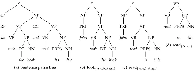
if the leaves of the subtree rooted inacorrespond to all and only the words of one argument ofp(i. e.,aexactly covers an argument), addφ(p,a) inE+(positive examples), otherwise add it inE−(negative examples).For instance, given the example in Figure 2(a), we would consider all the pairsp,a wherepis the node associated with the predicatetookandais any other tree node not overlapping with p. If the nodeaexactly covers the word sequencesJohn orthe book, thenφ(p,a) is added to the setE+, otherwise it is added toE−, as in the case of the node (NN book).
Figure 2
Positive (framed) and negative (unframed) examples of candidate argument nodes for the propositions (a) [Arg0John]took[Arg1the book]and read its titleand (b) [Arg0John]took the
book andread[Arg1its title].
ican be trained. We adopted this solution following Pradhan, Hacioglu, Krugler et al. (2005) because it is simple and effective. In the classification phase, given an unseen sentence, all the pairsp,aare generated and classified by each individual role classifier Ci. The argument label associated with the maximum among the scores provided byCi
is eventually selected.
The feature extraction functionφ can be implemented according to different lin-guistic theories and intuitions. From a technical point of view, we can useφ to map
p,a in feature vectors or in structures to be used in a tree kernel function. The next section describes our choices in more detail.
4.2 Linear and Structured Representation
Our feature extractor module and our learning algorithms are designed to cope with both linear and structured features, used for the different stages of the SRL process.
The standard features that we adopted are shown in Table 1. They include:
r
thePhrase Type,Predicate Word,Head Word,Governing Category,Position,andVoicedefined in Gildea and Jurafsky (2002);
r
thePartial Path,No Direction Path,Constituent Tree Distance,Head Word POS,First and Last Word/POS,Verb Subcategorization, andHead Word of the Noun Phrase in the Prepositional Phraseproposed in Pradhan, Hacioglu, Krugler et al. (2005); andr
theSyntactic Framedefined in Xue and Palmer (2004).We indicate with structured features the basic syntactic structures extracted from the sentence-parse tree or their canonical transformation (see Section 3.1). In particular, we focus on the minimal spanning tree that includes the predicate along with all of its arguments.
More formally, given a parse treet, a node set spanning tree(NST) over a set of nodesNt={n1,. . .,nk}is a partial tree oftthat (1) is rooted at the deepest level and (2)
contains all and only the nodesni∈Nt, along with their ancestors and descendants. An
Figure 3
(a) A sentence parse tree, the correct ASTns associated with two different predicates (b,c), and (d)
a correct AS T1relative to the argument Arg1its titleof the predicateread.
ofn1,. . .,nk. Then, from the set of all the descendants ofr, we remove all the nodesnj
that: (1) do not belong toNtand (2) are neither ancestors nor descendants of any node
belonging toNt.
Because predicate arguments are associated with tree nodes, we can define the pred-icate argument spanning tree(ASTn) of a predicate argument node setAp={a1,. . .,an}
as the NST over these nodes and the predicate node, that is, the node exactly covering the predicate p.2 An ASTn corresponds to theminimalparse subtree whose leaves are
all and only the word sequences belonging to the arguments and the predicate. For example, Figure 3a shows the parse tree of the sentence: John took the book and read its title.took{ARG0,ARG1}andread{ARG0,ARG1}are two ASTnstructures associated with the two predicatestookandread, respectively, and are shown in Figure 3b and 3c.
For each predicate, only one NST is a valid ASTn. Careful manipulations of an ASTn
can be employed for those tasks that require a representation of the whole predicate– argument structure, for example, overlap resolution or proposition re-ranking.
It is worth noting that thepredicate–argument feature, or PAF in Moschitti (2004), is a canonical transformation of the ASTn in the subtree including the predicatepand
only one of its arguments. For the sake of uniform notation, PAF will be referred to as AST1(argument spanning tree), the subscript1stressing the fact that the structure only encompasses one of the predicate arguments. An example AST1is shown in Figure 3d. Manipulations of an AST1structure can lead to interesting tree kernels for local learning tasks, such as boundary detection and argument classification.
Regardless of the adopted feature space, our multiclassification approach suffers from the problem of selecting both boundaries and argument roles independently of the whole structures. Thus, it is possible that (a) two labeled nodes refer to the same arguments (node overlaps) and (b) invalid role sequences are generated (e. g., Arg0, Arg0, Arg0, . . .). Next, we describe our approach to solving such problems.
4.3 Conflict Resolution
We call a conflict, or ambiguity, or overlap resolution a stage of the SRL process which resolves annotation conflicts that invalidate the underlying linguistic model. This
happens, for example, when both a node and one of its descendants are classified as positive boundaries, namely, they received a role label. We say that such nodes are
overlappingas their leaf (i. e., word) sequences overlap. Because this situation is not allowed by the PropBank annotation definition, we need a method to select the most appropriate word sequence. Our system architecture can employ one of three different
disambiguationstrategies:
r
a basic solution which, given two overlapping nodes, randomly selects one to be removed;r
the following heuristics:1. The node causing the major number of overlaps is removed, for example, a node which dominates two nodes labeled as arguments 2. Core arguments (i. e., arguments associated with the
subcategorization frame of the target verb) are always preferred over adjuncts (i. e., arguments that are not specific to verbs or verb senses)
3. In case the two previous rules do not eliminate all conflicts, the nodes located deeper in the tree are discarded; and
r
a tree kernel–based overlap resolution strategy consisting of an SVM trained to recognize non-clashing configurations that often correspond to correct propositions.The latter approach consists of: (1) a software module that generates all the possible non-overlapping configurations of nodes. These are built using the output of the local node classifiers by generating all the permutations of argument nodes of a predicate and re-moving the configurations that contain at least one overlap; (2) an SVM trained on such non-overlapping configurations, where the positive examples are correct predicate– argument structures (although eventually not complete) and negative ones are not. At testing time, we classify all the alternative non-clashing configurations. In case more than one structure is selected as correct, we choose the one associated with the highest SVM score.
These disambiguation modules can be invoked after either the BC or the RM classifi-cation. The different information available after each phase can be used to design differ-ent kinds of features. For example, the knowledge of the candidate role of an argumdiffer-ent node can be a key issue in the design of effective conflict resolution methodologies, for example, by eliminating ArgX, ArgX, ArgX, . . . sequences. These different approaches are discussed in Section 5.2.
The next section describes a more advanced approach that can eliminate overlaps and choose the most correct annotation for a proposition among a set of alternative labeling schemes.
4.4 A Joint Model for Re-Ranking
an algorithm to evaluate the most likely labeling schemes for a given predicate, and (2) a re-ranker that sorts the labeling schemes according to theircorrectness.
Step 1 uses the probabilities associated with each possible annotation of parse tree nodes, hence requiring a probabilistic output from BC and RM. As the SVM learning algorithm produces metric values, we applied Platt’s algorithm (Platt 1999) to convert them into probabilities, as already proposed in Pradhan, Ward et al. (2005). These posterior probabilities are then combined to generate then labelings that maximize a likelihood measure. Step 2 requires the training of an automatic re-ranker. This can be designed using a binary classifier that, given two annotations, decides which one is more accurate. We modeled such a classifier by means of three different kernels based on standard features, structured features, and their combination.
4.4.1 Evaluation of the N-best Annotations.First, we converted the output of each node-classifier into a posterior probability conditioned by its output scores (Platt 1999). This method uses a parametric model to fit onto a sigmoid distribution the posterior probability P(y=1,f), where f is the output of the classifier and the parameters are dynamically adapted to give the best probability output.3 Second, we selected then most likely sequences of node labelings. Given a predicate, the likelihood of a labeling scheme (orstate)sfor theKcandidate argument nodes is given by:
p(s)= K
i=1
pi(l), pi(l)= pi(li)pi(ARG) ifli=NARG (1−pi(ARG))2 otherwise
(2)
wherepi(l) is the probability of nodeibeing assigned the labell, andpi(l) is the same
probability weighted by the probabilitypi(ARG) of the node being an argument. Ifl=
NARG (not an argument) then both terms evaluate to (1−pi(ARG)) and the likelihood
of the NARG label assignment is given by (1−pi(ARG))2.
To select the n states associated with the highest probability, we cannot evaluate the likelihood of all possible states because they are exponential in number. In order to reduce the search space we (a) limit the number of possible labelings of each node to mand (b) avoid traversing all the states by applying a Viterbi algorithm to search for the most likely labeling schemes. From each state we generate the states in which a candidate argument is assigned different labels. This operation is bound to output at mostnstates which are generated by traversing a maximum ofn×mstates. Therefore, in the worst case scenario the number of traversed states isV=n×m×k,kbeing the number of candidate argument nodes in the tree.
During the search we also enforce overlap resolution policies. Indeed, for any given state in which a node nj is assigned a labell=NARG, we generate all; and only the
states in which all the nodes that are dominated bynjare assigned the NARG label.
4.4.2 Modeling an Automatic Re-Ranker.The Viterbi algorithm generates thenmost likely annotations for the proposition associated with a predicatep. These can be used to build annotation pairs,si,sj, which, in turn, are used to train a binary classifier that decides if
siis more accurate thatsj. Each candidate propositionsican be described by a structured
featuretiand a vector of standard featuresvi. As a whole, an exampleeiis described by
the tuplet1i,t2i,v1i,v2i, wheret1i andv1i refer to the first candidate annotation, whereast2i andv2i refer to the second one. Given such data, we can define the following re-ranking kernels:
Ktr(e1,e2)=Kt(t11,t 1
2)+Kt(t21,t 2
2)−Kt(t11,t 2
2)−Kt(t21,t 1 2) Kpr(e1,e2)=Kp(v11,v
1
2)+Kp(v21,v 2
2)−Kp(v11,v 2
2)−Kp(v21,v 1 2)
whereKtis one of the tree kernel functions defined in Section 3 andKpis a polynomial
kernel applied to the feature vectors. The final kernel that we use is the following combination:
K(e1,e2)=
Ktr(e1,e2)
|Ktr(e1,e2)|
+ Kpr(e1,e2)
|Kpr(e1,e2)|
Previous sections have shown how our SRL architecture exploits tree kernel func-tions to a large extent. In the next section, we describe in more detail our structured features and the engineering methods applied for the different subtasks of the SRL process.
5. Structured Feature Engineering
Structured features are an effective alternative tostandardfeatures in many aspects. An important advantage is that the target feature space can be completely changed even by small modifications of the applied kernel function. This can be exploited to identify features relevant to learning problems lacking a clear and sound linguistic or cognitive justification.
As shown in Section 3.1, a kernel function is a scalar productφ(o1)·φ(o2), where
φis a mapping in an Euclidean space, ando1 ando2 are the target data, for example, parse trees. To make the engineering process easier, we decomposeφinto acanonical mapping,φM, and a feature extractionfunction, φS, over the set of incoming parse trees. φM transforms a tree into a canonical structure equivalent to an entire class of input parses andφSshatters an input tree into its subparts (e. g., subtrees, subset trees, or partial trees as described in Section 3). A large number of different feature spaces can thus be explored by suitable combinationsφ=φS◦φMof mappings.
We study different canonical mappings to capture syntactic/semantic aspects useful for SRL. In particular, we define structured features for the different phases of the SRL process, namely, boundary detection, argument classification, conflict resolution, and proposition re-ranking.
5.1 Structures for Boundary Detection and Argument Classification
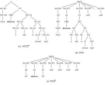
Figure 4
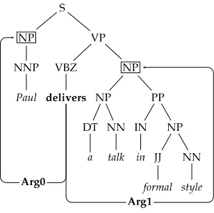
Parse tree of the example proposition [Arg0Paul]delivers[Arg1a talk in formal style].
Figure 5
(a) AST1, (b) ASTm1, and (c) AS Tcm1 structures relative to the argument Arg1a talk in formal styleof the predicatedeliversof the example parse tree shown in Figure 4.
specify the node that exactly covers the target argument node by simply marking it (or marking all its descendants) with the labelB, denoting the boundary property.
For example, Figure 4 shows the parse tree of the sentence Paul delivers a talk in formal style, highlighting the predicate with its two arguments, that is, Arg0 and Arg1. Figure 5 shows the AST1, AS Tm1, and ASTcm1 , that is, the basic structure, the structure with the marked argument node, and the completely marked structure, respectively.
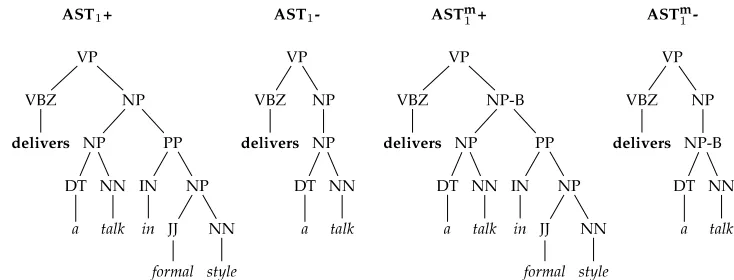
To understand the usefulness of node-marking strategies, we can examine Figure 6. This reports the case in which a correct and an incorrect argument node are chosen by also showing the corresponding AST1and ASTm1 representations ((a) and (b)). Figure 6c shows that the number of common fragments of two AST1 structures is 14. This is much larger than the number of common ASTm1 fragments, that is, only 3 substructures (Figure 6d).
Additionally, because the type of a target argument strongly depends on the type and number of the other predicate arguments4 (Punyakanok et al. 2005; Toutanova,
[image:17.486.57.435.256.394.2]Figure 6
(a) AST1s and (b) AS Tm1s extracted for the same target argument with their respective (c,b) common fragment spaces.
Haghighi, and Manning 2005), we should extract features from the whole predicate argument structure. In contrast, AST1s completely neglect the information (i. e., the tree portions) related to non-target arguments.
One way to use this further information with tree kernels is to use the minimum subtree that spans all the predicate–argument structures, that is, the ASTn defined in
Section 4.2.
However, ASTns pose two problems. First, we cannot use them for the boundary
detection task since we do not know the predicate–argument structure yet. We can derive the ASTn (its approximation) from the nodes selected by a boundary classifier, that is, the nodes that correspond to potential arguments. Such approximated ASTns
can be easily used in the argument classification stage.
Second, an ASTnis the same for all the arguments in a proposition, thus we need a
way to differentiate it for each target argument. Again, we can mark the target argument node as shown in the previous section. We refer to this subtree as a marked target
ASTn (ASTmtn ). However, for large arguments (i. e., spread over a large part of the
sentence tree) the substructures’ likelihood of being part of different arguments is quite high.
To address this problem, we can mark all the nodes that descend from the target argument node. We refer to this structure as acompletely marked targetASTn(ASTcmtn ).
5.2 Structured Features for Conflict Resolution
This section describes structured features employed by the tree kernel–based conflict resolution module of the SRL architecture described in Section 4.3. This subtask is performed by means of:
1. A first annotation of potential arguments using a high recall boundary classifier and, eventually, the role information provided by a role multiclassifier (RM).
2. An ASTnclassification step aiming at selecting, among the substructures
that do not contain overlaps, those that are more likely to encode the correct argument set.
The set of argument nodes recognized by BC can be associated with a subtree of the corresponding sentence parse, which can be classified using tree kernel functions. These should evaluate whether a subtree encodes a correct predicate–argument structure or not. As it encodes features from the whole predicate–argument structure, the ASTnthat
we introduced in Section 4.2 is a structure that can be employed for this task.
LetAp be the set of potential argument nodes for the predicatepoutput by BC; the
classifier examples are built as follows: (1) we look for node pairs n1,n2 ∈Ap×Ap
[image:19.486.54.383.424.623.2]wheren1 is the ancestor ofn2 orvice versa; (2) we create two node setsA1=A− {n1} andA2=A− {n2}and classify the two NSTs associated withA1 andA2 with the tree kernel classifier to select the most correct set of argument boundaries. This procedure can be generalized to a set of overlapping nodesOwith more than two elements, as we simply need to generate all and only the permutations ofA’s nodes that do not contain overlapping pairs.
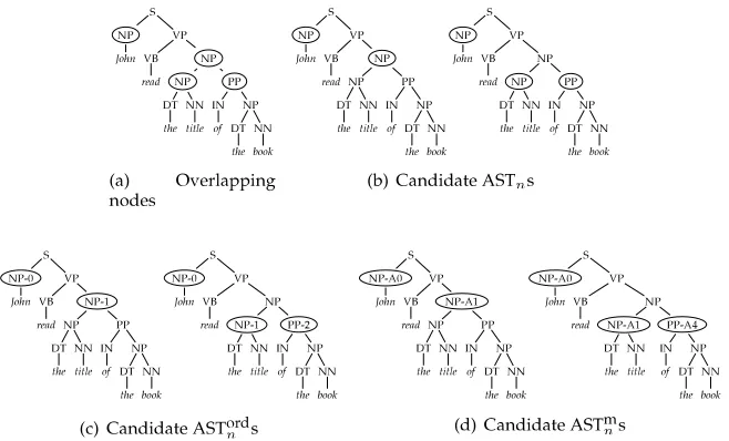
Figure 7 shows a working example of such a multi-stage classifier. In (Figure 7a), the BC labels as potential arguments four nodes (circled), three of which are overlapping
Figure 7
(in bold circles). The overlap resolution algorithm proposes two solutions (Figure 7b) of which only one is correct. In fact, according to the second solution, the preposi-tional phrase of the book would incorrectly be attached to the verbal predicate, that is, in contrast with the parse tree. The ASTn classifier, applied to the two NSTs,
should detect this inconsistency and provide the correct output. Figure 7 also high-lights a critical problem the ASTn classifier has to deal with: as the two NSTs are perfectly identical, it is not possible to distinguish between them using only their fragments.
In order to engineer novel features, we simply add the boundary information pro-vided by BC to the NSTs. We mark with a progressive number the phrase type cor-responding to an argument node, starting from the leftmost argument. We call the resulting structure an ordinal predicate–argument spanning tree (ASTordn ). For example, in the first NST of Figure 7c, we mark asNP-0andNP-1the first and second argument nodes, whereas in the second NST, we have a hypothesis of three arguments on three nodes that we transform asNP-0,NP-1, andPP-2.
This simple modification enables the tree kernel to generate features useful for dis-tinguishing between two identical parse trees associated with different argument struc-tures. For example, for the first NST the fragments[NP-1 [NP PP]],[NP [DT NN]], and [PP [IN NP]]are generated. They no longer match with the fragments of the second NST[NP-0 [NP PP]],[NP-1 [DT NN]], and[PP-2 [IN NP]].
We also experimented with another structure, the marked predicate–argument spanning tree (ASTmn), in which each argument node is marked with a role label as-signed by a role multi-classifier (RM). Of course, this model requires a RM to classify all the nodes recognized by BC first. An example ASTmn is shown in Figure 7d.
5.3 Structures for Proposition Re-Ranking
In Section 4.4, we presented our re-ranking mechanism, which is inspired by the joint inference model described in Haghighi, Toutanova, and Manning (2005). Designing structured features for the re-ranking classifier is complex in many aspects. Unlike the other structures that we have discussed so far, the defined mappings should: (1) preserve as much information as possible about the whole predicate–argument structure; (2) focus the learning algorithm on the whole structure; and (3) be able to identify those small differences that distinguish more or less accurate labeling schemes. Among the possible solutions that we have explored, three are especially interesting in terms of accuracy improvement or linguistic properties, and are described hereinafter.
The ASTcmn (completely marked ASTn, see Figure 8a) is an ASTn in which each
argument node label is enriched with the role assigned to the node by RM. The la-bels of the descendants of each argument node are modified accordingly, down to pre-terminal nodes. The ASTcmtn is a variant of ASTcmn in which only the target is marked. Marking a node descendant is meant to force substructures matching only among homogeneous argument types. This representation should provide rich syn-tactic and lexical information about the parse tree encoding the predicate–argument structure.
Figure 8
Different representations of the same proposition.
of structures. This structure accommodates the predicate and all the arguments of an annotation in a sequence of seven slots.5 To each slot is attached an argument label to which in turn is attached the subtree rooted in the argument node. The predicate is represented by means of a pre-terminal node labeledrelto which the lemmatization of the predicate word is attached as a leaf node. In general, a proposition consists of m arguments, withm≤6, wheremvaries according to the predicate and the context. To guarantee that predicate structures with a different number of arguments are matched in the SST kernel function, we attach a dummy descendant markednullto the slots not filled by an argument.
The PAStl (type-only, lemmatized PAS, see Figure 8c) is a specialization of the PAS that only focuses on the syntax of the predicate–argument structure, namely, the type and relative position of each argument, minimizing the amount of lexical and syntactic information derived from the parse tree. The differences with the PASare that: (1) each slot is attached to a pre-terminal node representing the argument type and a terminal node whose label indicates the syntactic type of the argument; and (2) the predicate word is lemmatized.
The next section presents the experiments used to evaluate the effectiveness of the proposed canonical structures in SRL.
6. Experiments
The experiments aim to measure the contribution and the effectiveness of our proposed kernel engineering models and of the diverse structured features that we designed (Section 5). From this perspective, the role of feature extraction functions is not fundamental because the study carried out in Moschitti (2006a) strongly suggests that the SST (Collins and Duffy 2002) kernel produces higher accuracy than the PT kernel when dealing with constituent parse trees, which are adopted in our study.6 We then selected the SST kernel and designed the following experiments:
(a) A study of canonical functions based on node marking for boundary detection and argument classification, that is, ASTm1 (Section 6.2). Moreover, as the standard features have shown to be effective, we combined them with ASTm1 based kernels on the boundary detection and classification tasks (Section 6.2).
(b) We varied the amount of training data to demonstrate the higher generalization ability of tree kernels (Section 6.3).
(c) Given the promising results of kernel engineering, we also applied it to solve a more complex task, namely, conflict resolution in SRL annotations (see Section 6.4). As this involves the complete predicate–argument structure, we could test advanced canonical functions generating ASTn, AS Tordn , and ASTmn.
(d) Previous work has shown that re-ranking is very important in boosting the accuracy of SRL. Therefore, we tested advanced canonical mappings, that is, those based on ASTcmn , PAS, and PAStl, on such tasks (Section 6.5).
6.1 General Setup
The empirical evaluations were mostly carried out within the setting defined in the CoNLL 2005 shared task (Carreras and M `arquez 2005). As a target data set, we used the PropBank7 and the automatic Charniak parse trees of the sentences of Penn TreeBank 2 corpus8(Marcus, Santorini, and Marcinkiewicz 1993) from the CoNLL 2005 shared-task data.9We employed the SVM-light-TK software10, which encodes fast tree kernel evaluation (Moschitti 2006b), and combinations between multiple feature vectors and trees in the SVM-light software (Joachims 1999). We used the default regularization parameter (option-c) andλ=0.4 (see Moschitti [2004]).
6.2 Testing Canonical Functions Based on Node Marking
In these experiments, we measured the impact of node marking strategies on boundary detection (BD) and the complete SRL task, that is, BD and role classification (RC). We employed a configuration of the architecture described in Section 4 and previously
6 Of course the PT kernel may be much more accurate in processing PASand PAStlbecause these are not simply constituent parse trees. Nevertheless, a study of the PT kernel potential is beyond the purpose of this article.
7http://www.cis.upenn.edu/∼ace.
8http://www.cis.upenn.edu/∼treebank.
9http://www.lsi.upc.edu/∼srlconll/.
Table 2
Number of arguments (Arguments) and of unrecoverable arguments (Unrecoverable) due to parse tree errors in Sections 2, 3, and 24 of the Penn TreeBank/PropBank.
Sec. Arguments Unrecoverable
2 198,373 454 (0.23%)
3 147,193 347 (0.24%)
[image:23.486.53.437.251.342.2]24 139,454 731 (0.52%)
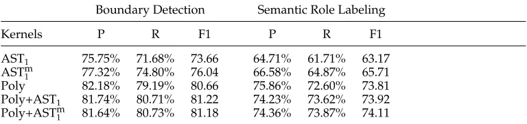
Table 3
Comparison between different models on Boundary Detection and the complete Semantic Role Labeling tasks. The training set is constituted by the first 1 million instances from Sections 02–06 for the boundary classifier and all arguments from Sections 02–21 for the role multiclassifier (253,129 instances). The performance is measured against Section 24 (149,140 instances).
Boundary Detection Semantic Role Labeling
Kernels P R F1 P R F1
AST1 75.75% 71.68% 73.66 64.71% 61.71% 63.17
ASTm1 77.32% 74.80% 76.04 66.58% 64.87% 65.71
Poly 82.18% 79.19% 80.66 75.86% 72.60% 73.81
Poly+AST1 81.74% 80.71% 81.22 74.23% 73.62% 73.92
Poly+ASTm1 81.64% 80.73% 81.18 74.36% 73.87% 74.11
adopted in Moschitti et al. (2005b), in which the simple conflict resolution heuristic is applied. The results were derived within the CoNLL setting by means of the related evaluator.
In more detail, in the BD experiments, we used the first million instances from the Penn TreeBank Sections 2–6 for training11and Section 24 for testing. Our classification model applied to this data replicates the results obtained in the CoNLL 2005 shared task, that is, the highest accuracy in BD among the systems using only one parse tree and one learning algorithm. For the complete SRL task, we used the previous BC and all the available data, that is, the sections from 2 to 21, for training the role multiclassifier.
It is worth mentioning that, as the automatic parse trees contain errors, some arguments cannot be associated with any covering node; thus we cannot extract a tree representation for them. In particular, Table 2 shows the number of arguments (column 2) for sections 2, 3, and 24 as well as the number of arguments that we could not take into account (Unrecoverable) due to the lack of parse tree nodes exactly covering their word spans. Note how Section 24 of the Penn TreeBank (which is not part of the Charniak training set) is much more affected by this problem.
Given this setting, the impact of node marking can be measured by comparing the AST1and the ASTm1 based kernels. The results are reported in the rows AST1and ASTm1 of Table 3. Columns 2, 3, and 4 show their Precision, Recall, and F1 measure on BD and columns 5, 6, and 7 report the performance on SRL. We note that marking the argument
node simplifies the generalization process as it improves both tasks by about 3.5 and 2.5 absolute percentage points, respectively.
However, Row Poly shows that the polynomial kernel using state-of-the-art fea-tures (Moschitti et al. 2005b) outperforms ASTm1 by about 4.5 percentage points in BD and 8 points in the SRL task. The main reason is that the employed tree structures do not explicitly encode very important features like the passive voice or predicate position. In Moschitti (2004), these are shown to be very effective especially when used in polynomial kernels. Of course, it is possible to engineer trees including these and other standard features with a canonical mapping, but the aim here is to provide new interesting representations rather than to abide by the simple exercise of representing already designed features within tree kernel functions. In other words, we follow the idea presented in Moschitti (2004), where tree kernels were suggested as a means to derive new features rather than generate a stand-alone feature set.
Rows Poly+AST1 and Poly+ASTm1 investigate this possibility by presenting the combination of polynomial and tree kernels. Unfortunately, the results on both BD and SRL do not show enough improvement to justify the use of tree kernels; for example, Poly+ASTm1 improves Poly by only 0.52 in BD and 0.3 in SRL. The small improvement is intuitively due to the use of (1) a state-of-the-art model as a baseline and (2) a very large amount of training data which decreases the contribution of tree features. In the next section an analysis in terms of training data will shed some light on the role of tree kernels for BD and RC in SRL.
6.3 The Role of Tree Kernels for Boundary Detection and Argument Classification
The previous section has shown that if a state-of-the-art model12 is adopted, then the tree kernel contribution is marginal. On the contrary, if a non state-of-the-art model is adopted tree kernels can play a significant role. To verify this hypothesis, we tested the polynomial kernel over the standard feature vector proposed in Gildea and Jurafsky (2002) obtaining an F1 of 67.3, which is comparable with the ASTm1 model, that is 65.71. Moreover, a kernel combination produced a significant improvement of both models reaching an F1 of 70.4.
Thus, the role of tree kernels relates to the design of features for novel linguistic tasks for which the optimal data representation has not yet been developed. For exam-ple, although SRL has been studied for many years and many effective features have been designed, representations for languages like Arabic are still not very well under-stood and raise challenges in the design of effective predicate–argument descriptions.
However, this hypothesis on the usefulness of tree kernels is not completely satis-factory as the huge feature space produced by them should play a more important role in predicate–argument representation. For example, the many fragments extracted by an AST1 provide a very promising back-off model for the Path feature, which should improve the generalization process of SVMs.
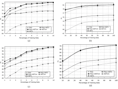
As back-off models show their advantages when the amount of training data is small, we experimented with Poly, AST1, AS Tm1, Poly+AST1, and Poly+ASTm1 and
different bins of training data, starting from a very small set, namely, 10,000 instances (1%) to 1 million (100%) of instances. The results from the BD classifiers and the complete SRL task are very interesting and are illustrated by Figure 9. We note several things.
First, Figure 9a shows that with only 1% of data (i.e., 640 arguments) as positive examples, the F1 on BD of the ASTm1 kernel is surprisingly about 3 percentage points higher than the one obtained by the polynomial kernel (Poly) (i. e., the state of the art). When ASTm1 is combined with Poly the improvement reaches 5 absolute percentage points. This suggests that tree kernels should always be used when small training data sets are available.
Second, although the performance of AST1is much lower than all the other models, its combination with Poly produces results similar to Poly+ASTm1, especially when the amount of training data increases. This, in agreement with the back-off property, indicates that the number of tree fragments is more relevant than their quality.
[image:25.486.54.440.325.616.2]Third, Figure 9b shows that as we increase training data, the advantage of using tree kernels decreases. This is rather intuitive as (i) in general less accurate data machine learning models trained with enough data can reach the accuracy of the most accurate models, and (ii) if the hypothesis that tree kernels provide back-off models is true, a lot of training data makes them less critical, for example, the probability of finding the Path feature of a test instance in the training set becomes high.
Figure 9
Table 4
Boundary detection accuracy (F1) on gold-standard parse trees and ambiguous structures employing the different conflict resolution methodologies described in Section 4.3.
RND HEU ASTordn
73.13 71.50 91.11
Finally, Figures 9c and 9d show learning curves13similar to Figures 9a and 9b, but with a reduced impact of tree kernels on the Poly model. This is due to the reduced impact of ASTm1 on role classification. Such findings are in agreement with the results in Moschitti (2004), which show that for argument classification the SCF structure (a variant of the ASTmn ) is more effective. Thus a comparison between learning curves of Poly and SCF on RC may show a behavior similar to Poly and ASTm1 for BD.
6.4 Conflict Resolution Results
In these experiments, we are interested in (1) the evaluation of the accuracy of our tree kernel–based conflict resolution strategy and (2) studying the most appropriate structured features for the task.
A first evaluation was carried out over gold-standard Penn TreeBank parses and PropBank annotations. We compared the alternative conflict resolution strategies imple-mented by our architecture (see Section 4.3), namely the random (RND), the heuristic (HEU), and a tree kernel–based disambiguator working with ASTordn structures. The disambiguators were run on the output of BC, that is, without any information about the candidate arguments’ roles. BC was trained on Sections 2 to 7 with a high-recall linear kernel. We applied it to classify Sections 8 to 21 and obtained 2,988 NSTs containing at least one overlapping node. These structures generated 3,624 positive NSTs (i. e., correct structures) and 4,461 negative NSTs (incorrect structures) in which no overlap is present. We used them to train the ASTordn classifier. The F1 measure on the boundary detection
task was evaluated on the 385 overlapping annotations of Section 23, consisting of 642 argument and 15,408 non-argument nodes.
The outcome of this experiment is summarized in Table 4. We note two points. (1) The RND disambiguator (slightly) outperforms the HEU. This suggests that the heuristics that we implemented were inappropriate for solving the problem. It also underlines how difficult it is to explicitly choose the aspects that are relevant for a complex, non-local task such as overlap resolution. (2) The ASTordn classifier outperforms the other strategies by about 20 percentage points, that is, 91.11 vs. 73.13 and 71.50. This datum along with the previous one is a good demonstration of how tree kernels can be effectively exploited to describe phenomena whose relevant features are largely unknown or difficult to represent explicitly. It should be noted that a more accurate baseline can be provided by using the Viterbi-style search (see Section 4.4.1). However, the experiments in Section 6.5 show that the heuristics produce the same accuracy (at least when the complete task is carried out).

![Figure 2Positive (framed) and negative (unframed) examples of candidate argument nodes for thebook andpropositions (a) [Arg0 John] took [Arg1 the book] and read its title and (b) [Arg0 John] took the read [Arg1 its title].](https://thumb-us.123doks.com/thumbv2/123dok_us/1271668.655229/12.486.50.352.62.196/figure-positive-negative-unframed-examples-candidate-argument-andpropositions.webp)